Spatial imports and standard workflow methods • scop

This page helps you choose the right input for a spatial method. First run the complete bundled Visium example: validate IDs and coordinates, calculate limited-assay QC, normalize without changing counts, inspect a real expression map, and save/reload the result. Then adapt the import section to an existing Visium, Visium HD, or Xenium vendor output directory.

The main spatial workflow provides the analysis path. The framework bridges page verifies conversion to SpatialExperiment and checks the optional Giotto backend.

Run a complete input check

visium_human_pancreas_sub comes from sample GSM8058244 (PanIN-LG2), study GSE254829. It contains all 1,986 packaged tissue spots and 5,000 genes shared with the bundled pancreas reference. The package has already selected those genes; this page does not reduce the object further. coda_label is supplied microanatomical annotation, not a predicted single-cell type.

library(scop)
data(visium_human_pancreas_sub)
visium <- visium_human_pancreas_sub
assay_name <- "Spatial"
image_name <- "slice1"
counts <- GetAssayData5(visium, assay = assay_name, layer = "counts")
raw_coordinates <- SpatialCoordinates(visium, image = image_name, space = "raw")

stopifnot(
  identical(dim(counts), c(5000L, 1986L)),
  !anyDuplicated(colnames(counts)),
  identical(rownames(visium@meta.data), colnames(visium)),
  setequal(colnames(counts), raw_coordinates$data$cell_id),
  all(is.finite(as.matrix(raw_coordinates$data[, c("x", "y")]))),
  all(is.finite(counts@x)), all(counts@x >= 0),
  all(counts@x == floor(counts@x))
)
input_receipt <- data.frame(
  source = "GSE254829 / GSM8058244 / complete bundled object",
  observations = ncol(counts), features = nrow(counts),
  observation_unit = "spot", assay = assay_name, layer = "counts",
  image = image_name, coordinate_space = "raw", coordinate_units = "pixel",
  total_selected_gene_counts = sum(counts)
)
input_receipt
#>                                             source observations features
#> 1 GSE254829 / GSM8058244 / complete bundled object         1986     5000
#>   observation_unit   assay  layer  image coordinate_space coordinate_units
#> 1             spot Spatial counts slice1              raw            pixel
#>   total_selected_gene_counts
#> 1                    8220223
raw_coordinates$source
#> $image
#> [1] "slice1"
#> 
#> $coord.cols
#> [1] "x" "y"
#> 
#> $image_policy
#> [1] "strict"
#> 
#> $coordinate_space
#> [1] "raw"
#> 
#> $image_class
#> [1] "VisiumV2"
#> attr(,"package")
#> [1] "Seurat"
#> 
#> $image_width
#> [1] 600
#> 
#> $image_height
#> [1] 340
#> 
#> $scale_name
#> [1] "lowres"
#> 
#> $scale_factor
#> [1] 0.078125
#> 
#> $coordinate_contract_version
#> [1] 3
SeuratObject::Layers(visium[[assay_name]])
#> [1] "counts"

The count total describes only the packaged genes. The ID checks prevent an expression column from being paired with another spot’s coordinates. The fixed dimension check is specific to this example; replace it with your own expected dimensions. Keep the general ID, finite-coordinate, and raw-count checks when changing datasets.

Label QC problems without discarding observations

A gene-filtered assay cannot reproduce whole-transcriptome library complexity or mitochondrial percentages. Here, UMI and gene thresholds are an executable example on the retained genes, not validated tissue-QC cutoffs. For real QC, import the complete raw expression assay and choose thresholds after examining its distributions and tissue image.

qc_parameters <- list(qc_metrics = c("umi", "gene"), UMI_threshold = 500,
                      gene_threshold = 200, return_filtered = FALSE)
visium_qc <- do.call(RunSpotQC, c(
  list(object = visium, assay = assay_name, verbose = FALSE), qc_parameters
))
qc_summary <- as.data.frame(table(visium_qc$SpotQC, useNA = "ifany"))
colnames(qc_summary) <- c("status", "spots")
qc_summary
#>   status spots
#> 1   Pass  1957
#> 2   Fail    29
summary(visium_qc@meta.data[, c("nCount_Spatial", "nFeature_Spatial")])
#>  nCount_Spatial  nFeature_Spatial
#>  Min.   :   36   Min.   :  32    
#>  1st Qu.: 1865   1st Qu.:1157    
#>  Median : 3370   Median :1796    
#>  Mean   : 4139   Mean   :1873    
#>  3rd Qu.: 6051   3rd Qu.:2604    
#>  Max.   :18957   Max.   :4232
stopifnot(
  identical(colnames(visium_qc), colnames(visium)),
  isTRUE(all.equal(GetAssayData5(visium_qc, assay = assay_name, layer = "counts"), counts)),
  sum(qc_summary$spots) == ncol(visium)
)

Pass means both requested thresholds passed; Fail means at least one failed. An NA result is unresolved, not a pass. All observations remain in this example because return_filtered = FALSE, so you can inspect failures before deciding whether to exclude them.

SpatialSpotPlot(visium_qc, group.by = "SpotQC", image = image_name)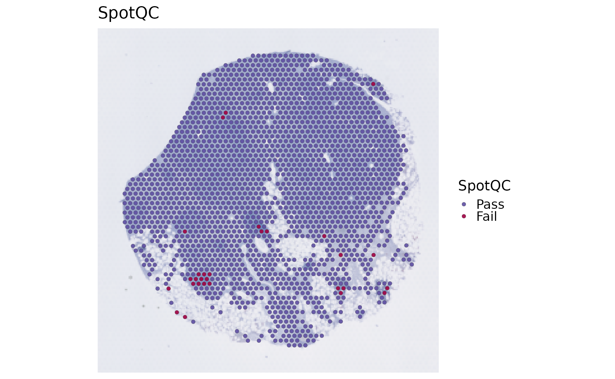

Normalize and inspect a measured feature

visium_normalized <- Seurat::NormalizeData(
  visium_qc, assay = assay_name, normalization.method = "LogNormalize",
  scale.factor = 10000, verbose = FALSE
)
stopifnot(isTRUE(all.equal(
  GetAssayData5(visium_normalized, assay = assay_name, layer = "counts"), counts
)))
SeuratObject::Layers(visium_normalized[[assay_name]])
#> [1] "counts" "data"
feature <- "GCG"
stopifnot(feature %in% rownames(counts))
feature_values <- GetAssayData5(visium_normalized, assay = assay_name, layer = "data")[feature, ]
data.frame(feature = feature, spots_with_counts = sum(counts[feature, ] > 0),
           minimum_log_expression = min(feature_values),
           maximum_log_expression = max(feature_values))
#>   feature spots_with_counts minimum_log_expression maximum_log_expression
#> 1     GCG              1861                      0               7.154526

SpatialSpotPlot(visium_normalized, features = feature, assay = assay_name,
                layer = "data", image = image_name, palette = "YlGnBu",
                legend.title = "Log-normalized GCG")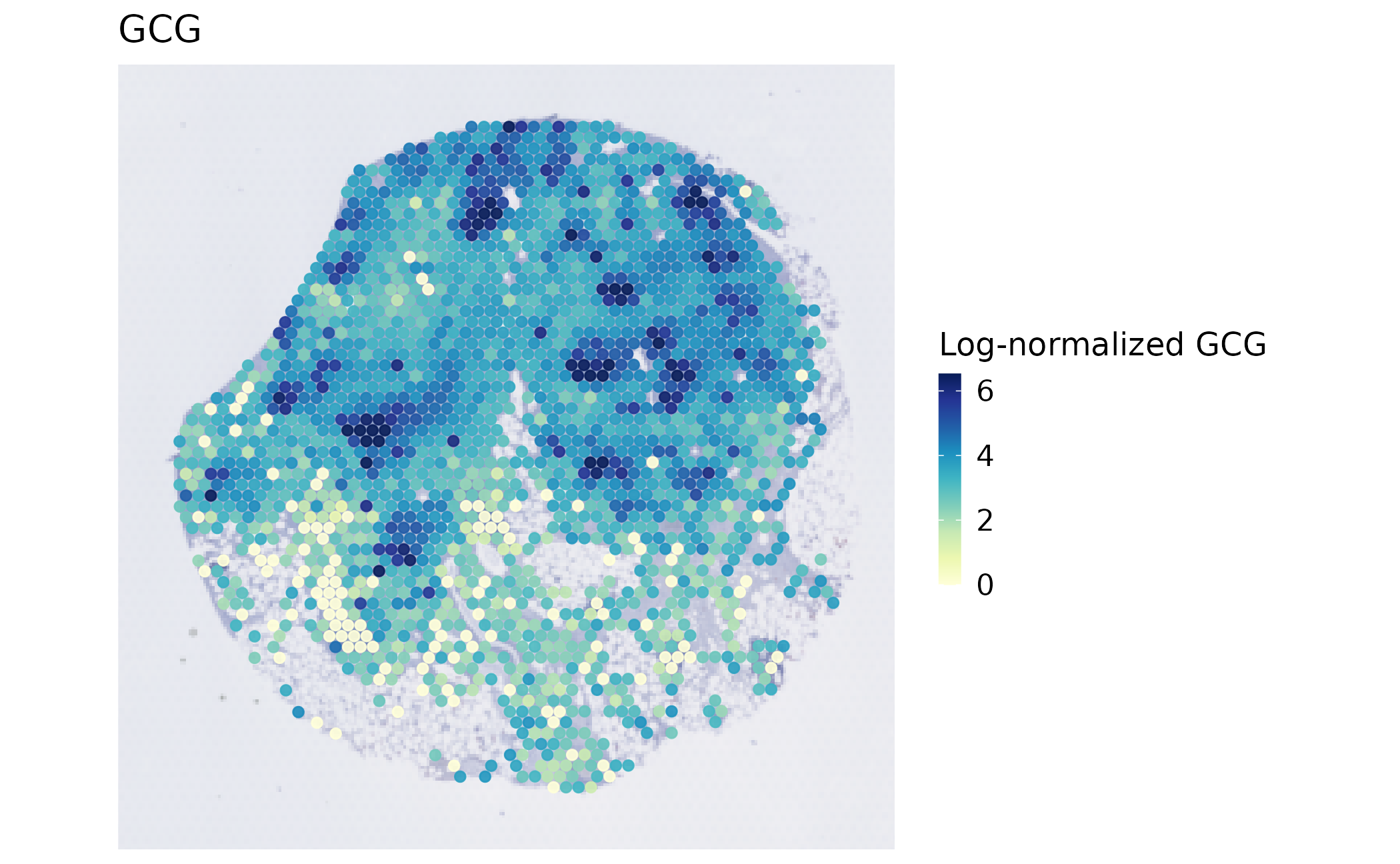

This map shows measured GCG expression after library-size scaling and log1p transformation over the retained genes. It is not a deconvolution result or a cell-type call. Recompute normalization from a complete assay for production analysis; values normalized over different gene universes need not be comparable. The counts equality check confirms that the raw source was preserved.

Save, reload, and verify

output_dir <- Sys.getenv("SCOP_PLATFORM_OUTPUT_DIR", file.path(tempdir(), "scop-platform"))
dir.create(output_dir, recursive = TRUE, showWarnings = FALSE)
result_file <- file.path(output_dir, "panin-input-qc-normalized.rds")
saveRDS(list(object = visium_normalized, input = input_receipt,
             qc_parameters = qc_parameters, qc_summary = qc_summary,
             coordinates = raw_coordinates, session = utils::sessionInfo()), result_file)
reloaded <- readRDS(result_file)
reload_checks <- c(
  observations = identical(colnames(reloaded$object), colnames(visium)),
  counts = isTRUE(all.equal(
    GetAssayData5(reloaded$object, assay = assay_name, layer = "counts"), counts)),
  qc_labels = identical(reloaded$object$SpotQC, visium_normalized$SpotQC),
  coordinates = identical(
    SpatialCoordinates(reloaded$object, image = image_name, space = "raw"), raw_coordinates)
)
data.frame(check = names(reload_checks), passed = unname(reload_checks))
#>          check passed
#> 1 observations   TRUE
#> 2       counts   TRUE
#> 3    qc_labels   TRUE
#> 4  coordinates   TRUE
stopifnot(all(reload_checks))

The build writes to a temporary directory. Set SCOP_PLATFORM_OUTPUT_DIR to a new persistent project directory before running this code on your data. Use reloaded$object in either plotting call above; plotting does not rerun QC or normalization. Save the input receipt alongside figures so their units and selected assay remain recoverable.

Platform contracts at a glance

Input	Observation	Typical assay/image	Coordinate meaning	Natural SCOP entry
Visium	spot	`Spatial` / `slice1`	full-resolution image pixels; display scale is separate	`SpatialSpotPlot()`, spot QC, Moran/Geary, domain clustering, spot deconvolution
Visium HD	bin	`Spatial.008um` or `Spatial.016um` / matching image	full-resolution pixels for the selected bin resolution	`SpatialSpotPlot()`, resolution-aware BayesSpace, spatial-variable features
Xenium	segmented cell	vendor assay / `fov`	vendor segmentation coordinates in microns	`SpatialCellPlot()`, cell-level context or communication

The exact assay and image names are read from the loaded object; do not copy a name from a different resolution or sample. Check the selected context before calling a method:

SpatialCoordinates(visium, image = image_name, space = "raw")$source
#> $image
#> [1] "slice1"
#> 
#> $coord.cols
#> [1] "x" "y"
#> 
#> $image_policy
#> [1] "strict"
#> 
#> $coordinate_space
#> [1] "raw"
#> 
#> $image_class
#> [1] "VisiumV2"
#> attr(,"package")
#> [1] "Seurat"
#> 
#> $image_width
#> [1] 600
#> 
#> $image_height
#> [1] 340
#> 
#> $scale_name
#> [1] "lowres"
#> 
#> $scale_factor
#> [1] 0.078125
#> 
#> $coordinate_contract_version
#> [1] 3
SeuratObject::DefaultAssay(visium)
#> [1] "Spatial"
SeuratObject::Images(visium)
#> [1] "slice1"

SCOP keeps spot IDs/cell IDs aligned with expression columns. If several images cover one sample, analysis and plotting require an explicit selection or an explicit named sample-to-image map. A display lowres/hires scale never changes raw distances and does not turn pixels into microns.

Import existing vendor output

Set one or more of SCOP_VISIUM_DIR, SCOP_VISIUM_HD_DIR, and SCOP_XENIUM_DIR to existing, unpacked vendor output directories before running this section. Visium needs the expression matrix plus the spatial/ outputs; HD needs the selected binned outputs and matching images; Xenium needs expression and existing cell segmentation. Do not point at an archive. No path is configured by default, so the table explicitly reports not_run.

vendor_paths <- c(
  visium = Sys.getenv("SCOP_VISIUM_DIR"),
  visium_hd = Sys.getenv("SCOP_VISIUM_HD_DIR"),
  xenium = Sys.getenv("SCOP_XENIUM_DIR")
)
vendor_objects <- list()
import_receipts <- lapply(names(vendor_paths), function(technology) {
  path <- vendor_paths[[technology]]
  status <- "not_run"
  reason <- "No vendor directory configured"
  observations <- NA_integer_
  if (nzchar(path)) {
    result <- tryCatch({
      if (!dir.exists(path)) stop("Configured vendor directory does not exist")
      ReadSpatialData(data.dir = path, technology = technology,
                      bin.size = c(8, 16), sample_id = paste0(technology, "_sample1"))
    }, error = function(e) e)
    if (inherits(result, "error")) {
      status <- "failed"
      reason <- conditionMessage(result)
    } else {
      vendor_objects[[technology]] <<- result
      status <- "completed"
      reason <- "Vendor import and SCOP context validation completed"
      observations <- ncol(result)
    }
  }
  data.frame(technology = technology, status = status, observations = observations,
             reason = reason)
})
import_receipts <- do.call(rbind, import_receipts)
import_receipts
#>   technology  status observations                         reason
#> 1     visium not_run           NA No vendor directory configured
#> 2  visium_hd not_run           NA No vendor directory configured
#> 3     xenium not_run           NA No vendor directory configured

Only completed means an import ran. For example, after a successful Visium import, use visium <- vendor_objects$visium, inspect its images/assays, and repeat the input checks with its actual dimensions. If your matrix filename is nonstandard, pass Seurat’s filename = argument through ReadSpatialData(); the GSE254829 source archive uses filename = "filtered_feature_bc_matrix". For HD, inspect every image and its matching assay separately: one resolution is not interchangeable with another.

ReadSpatialData() delegates file parsing to Seurat and records import provenance under object@misc$scop_spatial_input. It validates that each returned image, assay, observation set, resolution, and coordinate-unit label agree. It does not normalize counts, segment cells, or infer cell types.

Public data sources for testing the input formats are available from the 10x Genomics Visium datasets, the 10x Visium HD human-pancreas example, the 10x Visium HD developer example data, and 10x Xenium Explorer demo datasets. Download and unpack them outside the package; do not hard-code a machine path in a reproducible article.

Optional method recipes: check availability first

The complete input/QC/normalization path above is evaluated. The following backend-specific recipes are not executed by this page: several require separate installations, another sample, a matched reference, or a costly model fit. This table measures installation status and explicitly distinguishes it from execution. A package being installed does not prove that its model ran.

backend_packages <- c("SpaNorm", "Banksy", "BayesSpace", "PRECAST", "spacexr")
backend_status <- data.frame(
  package = backend_packages,
  installed = vapply(backend_packages, requireNamespace, logical(1), quietly = TRUE),
  version = vapply(backend_packages, function(p) {
    if (requireNamespace(p, quietly = TRUE)) as.character(packageVersion(p)) else NA_character_
  }, character(1)),
  execution = "not_run: optional recipe on this page"
)
backend_status
#>               package installed version                             execution
#> SpaNorm       SpaNorm      TRUE   1.6.0 not_run: optional recipe on this page
#> Banksy         Banksy      TRUE   1.8.1 not_run: optional recipe on this page
#> BayesSpace BayesSpace      TRUE  1.22.0 not_run: optional recipe on this page
#> PRECAST       PRECAST      TRUE     1.9 not_run: optional recipe on this page
#> spacexr       spacexr      TRUE   2.2.1 not_run: optional recipe on this page

The main workflow contains executable spatial-feature and reference-based examples. Use its execution receipts to establish which methods actually ran.

Visium and Visium HD: keep counts and normalized data separate

Raw counts are the input for count-dependent QC and methods that model sampling depth. Normalized/log-transformed data are appropriate for expression-level plots and methods whose contract asks for a normalized layer. SpaNorm is a separate normalization stage; it does not replace the original count source.

stopifnot(requireNamespace("SpaNorm", quietly = TRUE),
          requireNamespace("Banksy", quietly = TRUE))
normalized <- RunStandardWorkflow(
  visium,
  workflow = "spatial",
  assay = "Spatial",
  image = "slice1",
  normalization_method = "SpaNorm",
  spot_qc_params = qc_parameters,
  spanorm_params = list(new_assay = "SpaNormAnalysis"),
  do_spatial_cluster = TRUE,
  spatial_cluster_method = "BANKSY",
  do_deconvolution = FALSE
)

normalized@tools$run_standard_spatial_workflow$stages

# A separate count-dependent method; q is a required choice, not an inferred truth.
stopifnot(requireNamespace("BayesSpace", quietly = TRUE))
bayesspace <- RunBayesSpace(
  normalized,
  assay = "Spatial",  # this assay must retain the original counts
  image = "slice1",
  q = 4,
  store_sce = FALSE
)
table(bayesspace$BayesSpace_cluster)

The workflow attaches matching original counts when needed for QC and uses the separate normalized assay for downstream expression preprocessing. It rejects an explicit do_normalization = FALSE conflict with SpaNorm. Do not relabel normalized values as counts. RunBayesSpace() has no layer argument: its selected assay must contain the intended counts. Inspect the domain map and compare justified choices of q; four domains in this recipe is a parameter, not a biological conclusion.

Standard methods by platform

For a Visium spot or HD bin, a compact method selection is:

baseline <- RunStandardWorkflow(
  visium,
  workflow = "spatial",
  assay = "Spatial",
  image = "slice1",
  do_spot_qc = TRUE,
  spot_qc_params = qc_parameters,
  do_spatial_variable_features = TRUE,
  spatial_variable_features_params = list(method = "moran", nfeatures = nrow(visium[["Spatial"]])),
  do_spatial_cluster = FALSE,
  do_deconvolution = FALSE
)

baseline@tools$run_standard_spatial_workflow$stages
stopifnot(requireNamespace("Banksy", quietly = TRUE))
banksy <- RunStandardWorkflow(
  visium,
  workflow = "spatial",
  assay = "Spatial",
  image = "slice1",
  do_spot_qc = FALSE,
  do_spatial_variable_features = FALSE,
  do_spatial_cluster = TRUE,
  spatial_cluster_method = "BANKSY",
  spatial_cluster_params = list(lambda = 0.2, resolution = 0.6),
  do_deconvolution = FALSE
)

banksy@tools$run_standard_spatial_workflow$stages
table(banksy$BANKSY_cluster)
SpatialSpotPlot(banksy, group.by = "BANKSY_cluster", image = "slice1")

BayesSpace is the spot/bin array branch; spatial_q or BayesSpace’s q controls the number of domains. BANKSY uses its own resolution parameters. SmoothClust accepts a requested n_clusters and its smoothing parameters. Segmented cell observations are not silently sent through spot deconvolution or BayesSpace; use cell-level methods and plots instead.

Multi-sample PRECAST integration

Integration needs a sample label and a covering image per sample. With a merged object, the image map names are the merged object’s image keys. With list input, the map names refer to the original list element names before Seurat renames duplicate image keys.

Use two independently acquired samples saved as Seurat RDS files. Set the two environment variables below to those files; do not split or duplicate this single bundled section to manufacture an integration result. Inspect each object and adjust the assay/image map before running.

stopifnot(requireNamespace("PRECAST", quietly = TRUE))
sample_files <- c(S1 = Sys.getenv("SCOP_SPATIAL_S1_RDS"),
                  S2 = Sys.getenv("SCOP_SPATIAL_S2_RDS"))
stopifnot(all(nzchar(sample_files)), all(file.exists(sample_files)),
          length(unique(normalizePath(sample_files))) == 2L)
visium_S1 <- readRDS(sample_files[["S1"]])
visium_S2 <- readRDS(sample_files[["S2"]])
stopifnot(inherits(visium_S1, "Seurat"), inherits(visium_S2, "Seurat"))
lapply(list(S1 = visium_S1, S2 = visium_S2), SeuratObject::Images)

integrated <- RunSpatialIntegration(
  object = list(S1 = visium_S1, S2 = visium_S2),
  method = "PRECAST",
  assay = "Spatial",
  layer = "counts",
  image = c(S1 = "slice1", S2 = "slice1"),
  store_object = FALSE
)

integrated@tools$SpatialIntegration$summary
SeuratObject::Images(integrated)
SpatialIntegrationPlot(integrated, plot_type = "spatial")
saveRDS(integrated, "precast-integration.rds")

The plotting call resolves the images in the merged object. Inspect SeuratObject::Images(integrated) before supplying an explicit plotting map: duplicate input names such as slice1 may have been renamed during merging. Do not reuse the input-list map as a merged-object map.

The PRECAST package is an execution-time optional dependency. The template is not a successful run unless PRECAST is installed and the input objects exist. store_object = FALSE omits only the complete native PRECAST object; domains, embedding, aligned coordinates, parameters, source information, and standard plots remain stored. Keep the default TRUE when a later native PRECAST analysis needs the full object.

PRECAST receives a fresh backend object built from the selected assay and layer, which must contain finite, non-negative integer counts; it normalizes these counts internally. The default adjacency uses six nearest neighbors in the selected coordinate space (adj_params = list(type = "fixed_number", number = 6)). SCOP constructs this graph with its shared exact KNN implementation and adapts it to PRECAST’s column-neighbor matrix convention. Each sample must retain more spots than the requested neighbor count. PRECAST’s fixed-distance Visium/ST mode expects array indices and is rejected for SCOP’s analysis coordinates. Empty or invalid graphs stop before training. Effective backend arguments and per-sample nonzero edge counts are saved under the method bundle’s parameters.

For SpatialCellChat, verify the physical calibration before interpreting distance-dependent communication. The current wrapper has a legacy ordinary Visium fallback of 65 / spot_diameter_fullres and tol = 32.5; these are implementation assumptions, not the current platform specification. 10x specifies a 55-micron diameter for ordinary Visium spots. For confirmed 55-micron spots with full-resolution pixel coordinates, supply ratio = 55 / spot_diameter_fullres explicitly and choose a justified tol in microns. Do not apply a full-resolution ratio to resized-image coordinates. Visium HD needs its own calibrated ratio and tolerance for the chosen bin or cell size; an ordinary spot-diameter conversion does not apply. Imported HD provenance and assay names such as Spatial.008um inform automatic technology detection; an explicit technology = "visium_hd" is needed when that evidence is absent.

Deconvolution and cell2location storage choices

Spot deconvolution is reference-dependent and estimates composition per spot; it does not turn a spot into a segmented cell. RunRCTD(), RunSPOTlight(), and RunCell2location() preserve their own result semantics. Use SpatialDeconvolutionPlot() or Cell2locationPlot() after checking the stored result. Cell2location q05 abundance and normalized proportions are distinct; the abundance view uses its native range rather than a forced 0–1 scale. Cell2location plotting matrices retain the original spot IDs. Spots excluded from modeling, such as zero-count observations, have NA values rather than zero abundance. The saved cells field identifies modeled spots, and input_summary$dropped_spots records filtered observations. Historical compact results are expanded only when those records explain all missing rows; missing predictions or unknown IDs are not silently accepted. An explicit lower_cutoff, upper_cutoff, or quantile control overrides the default matrix-wide display range. With a one-sided override, each panel keeps the remaining bound computed by SpatialSpotPlot(); specify both cutoffs when you want identical explicit limits across panels. combine changes only the return form, including for the dominant point map.

For a complete reference-backed RCTD run, use the main workflow. Choose a reference with compatible gene identifiers and biologically relevant labels, and retain its count assay. The stored model result, not an invented component matrix, is the input to SpatialDeconvolutionPlot(). For a saved cell2location result, verify that input_summary, modeled cells, and the selected abundance/proportion matrix are present before calling Cell2locationPlot().

Common errors and how to recover

Symptom	Check and recovery
Vendor directory does not exist or a matrix is missing	Unpack the archive; point at the vendor output directory; check the actual matrix filename and loader arguments
More than one image or HD resolution	List images and matching assays; select the intended pair explicitly, one resolution at a time
Image IDs are absent from the assay	Compare IDs and sample/resolution provenance; choose the matching assay instead of silently taking an intersection
QC labels are unexpectedly good or bad	Check the gene universe and count layer; inspect distributions and tissue; do not apply whole-transcriptome thresholds to a selected-gene assay
SpaNorm conflicts with normalization settings	Remove `do_normalization = FALSE` when requesting SpaNorm and preserve the original count assay
A backend is installed but no result is present	Read the actual workflow stage status/reason; package availability is not a completed analysis
PRECAST adjacency is empty or invalid	Verify raw coordinates, sample/image coverage, and more than six spots per sample for the default six-neighbor graph
Spots have missing composition values	Check the producer’s modeled cells and dropped-spot record; `NA` means unmodeled/missing, not zero abundance

Validation and analysis receipts

Acceptance runs use public slide data outside the package: developer fixtures check format and computation rather than biological performance on production slides, and public slide data are not redistributed with scop.

For a new dataset, preserve the following in the analysis receipt:

platform and observation unit (spot, bin, or cell);
assay and layer, selected image, coordinate columns, coordinate space, and physical units when known;
raw-count versus normalized-expression input decisions;
sample-to-image map for every sample;
stage status and backend versions for methods that actually ran.

data.frame(
  package = c("scop", "Seurat", "SeuratObject", "Matrix"),
  version = vapply(c("scop", "Seurat", "SeuratObject", "Matrix"),
                   function(p) as.character(utils::packageVersion(p)), character(1))
)
#>                   package version
#> scop                 scop   0.9.2
#> Seurat             Seurat   5.6.0
#> SeuratObject SeuratObject   5.4.0
#> Matrix             Matrix   1.7.5

Build provenance

This receipt belongs to the actual rendered source and retained observations. Save it beside the exported object when adapting the workflow.

source_revision <- Sys.getenv("GITHUB_SHA")
if (!nzchar(source_revision) && nzchar(Sys.which("git"))) {
  source_revision <- system2("git", c("rev-parse", "HEAD"), stdout = TRUE,
                             stderr = FALSE)[1]
}
build_receipt <- data.frame(
  article = "spatial-platform-workflows", built_utc = format(Sys.time(), tz = "UTC", usetz = TRUE),
  source_revision = source_revision,
  source_has_local_changes = if (nzchar(Sys.which("git")))
    length(system2("git", c("status", "--porcelain"), stdout = TRUE,
                   stderr = FALSE)) > 0 else NA,
  article_md5 = unname(tools::md5sum(knitr::current_input(dir = TRUE))),
  R = as.character(getRversion()), scop = as.character(utils::packageVersion("scop")),
  retained_observations = ncol(visium_normalized), genes = nrow(visium_normalized)
)
build_receipt
#>                      article               built_utc
#> 1 spatial-platform-workflows 2026-10-12 00:11:32 UTC
#>                            source_revision source_has_local_changes
#> 1 083f5f31e37220a9e9a5b0110e63ea4ed3f49317                    FALSE
#>                        article_md5     R  scop retained_observations genes
#> 1 857e67c53d4bc4a42ef8c52375db5a5d 4.6.1 0.9.2                  1986  5000
utils::write.csv(build_receipt, file.path(output_dir, "build-receipt.csv"), row.names = FALSE)
writeLines(capture.output(sessionInfo()), file.path(output_dir, "session-info.txt"))