Spatial domain benchmark workflow
Source:vignettes/spatial-benchmark-workflow.Rmd
spatial-benchmark-workflow.RmdThis article compares spatial domain clustering methods with [RunSpatialBenchmark()]. Each method runs in an isolated R process; results include ARI, NMI, purity, runtime, and peak memory against a gold-standard label column. Visualize the result with [SpatialBenchmarkPlot()].
Supported producers include BayesSpace,
BANKSY, and SmoothClust. This workflow is
separate from scRNA batch integration benchmarking
([RunIntegrationBenchmark()]).
Load data and define a gold standard
This workflow uses a small simulated spatial object with three regions and region-specific expression signals. It demonstrates the benchmark interface; replace the simulated labels with tissue annotations for real analyses.
library(scop)

set.seed(42)
n_spots <- 36L
n_genes <- 60L
grid <- expand.grid(x = 1:6, y = 1:6)
spatial_domain <- factor(ifelse(grid$x <= 2, "left", ifelse(grid$x <= 4, "middle", "right")))
counts <- matrix(rpois(n_genes * n_spots, 2),
  nrow = n_genes,
  dimnames = list(paste0("Gene", seq_len(n_genes)), paste0("spot", seq_len(n_spots)))
)
signal <- split(seq_len(n_genes), rep(c("left", "middle", "right"), each = 20))
for (label in names(signal)) {
  counts[signal[[label]], spatial_domain == label] <-
    counts[signal[[label]], spatial_domain == label] + rpois(sum(spatial_domain == label) * 20, 5)
}
spatial <- SeuratObject::CreateSeuratObject(counts)
#> Warning: Data is of class matrix. Coercing to dgCMatrix.
spatial$x <- grid$x
spatial$y <- grid$y
spatial$gold_domain <- spatial_domain
table(spatial$gold_domain)
#>
#>   left middle  right
#>     12     12     12
Run the benchmark
Methods share the same spot set. Tune per-method arguments through
method_params when backends need different PCA counts or
layers.
bench <- RunSpatialBenchmark(
  spatial,
  gold_standard = "gold_domain",
  method_params = list(
    BayesSpace = list(n.PCs = 5, n.HVGs = 20, coord.cols = c("x", "y")),
    BANKSY = list(layer = "counts", coord.cols = c("x", "y")),
    SmoothClust = list(layer = "counts", min_spots = 1, coord.cols = c("x", "y"))
  ),
  verbose = FALSE
)

bench$summary
#>        method      workflow ARI NMI purity runtime_s baseline_memory_mb
#> 1  BayesSpace SpatialDomain   1   1      1    11.683           624.6289
#> 2      BANKSY SpatialDomain  NA  NA     NA     3.776           624.4648
#> 3 SmoothClust SpatialDomain   1   1      1     3.361           624.9102
#>   peak_memory_mb memory_delta_mb n_evaluated n_clusters  status
#> 1      1252.3164        627.6875          36          3 success
#> 2       891.1484        266.6836           0         NA  failed
#> 3       876.3125        251.4023          36          3 success
#>                               error
#> 1
#> 2 Not enough neighbors in data set!
#> 3
Inspect the result object
RunSpatialBenchmark() returns a
spatial_benchmark_result list:
-
$summary: quality and resource metrics per method; -
$predictions: aligned domain labels per spot; -
$metrics: long metric table for custom plots.
str(bench$summary, max.level = 1)
#> 'data.frame':    3 obs. of  13 variables:
#>  $ method            : chr  "BayesSpace" "BANKSY" "SmoothClust"
#>  $ workflow          : chr  "SpatialDomain" "SpatialDomain" "SpatialDomain"
#>  $ ARI               : num  1 NA 1
#>  $ NMI               : num  1 NA 1
#>  $ purity            : num  1 NA 1
#>  $ runtime_s         : num  11.68 3.78 3.36
#>  $ baseline_memory_mb: num  625 624 625
#>  $ peak_memory_mb    : num  1252 891 876
#>  $ memory_delta_mb   : num  628 267 251
#>  $ n_evaluated       : int  36 0 36
#>  $ n_clusters        : int  3 NA 3
#>  $ status            : chr  "success" "failed" "success"
#>  $ error             : chr  "" "Not enough neighbors in data set!" ""
head(bench$predictions)
#>   spot_id gold_standard     method prediction
#> 1   spot1          left BayesSpace          1
#> 2   spot2          left BayesSpace          1
#> 3   spot3        middle BayesSpace          3
#> 4   spot4        middle BayesSpace          3
#> 5   spot5         right BayesSpace          2
#> 6   spot6         right BayesSpace          2
Plot benchmark views
For a spatial_benchmark_result,
plot_type = "auto" selects the publication-oriented
overview that combines clustering agreement with runtime and peak-memory
efficiency. For an ordinary summary table, auto selects the
stable native bar view; it does not depend on whether the optional
funkyheatmap package happens to be installed.
SpatialBenchmarkPlot(data = bench, plot_type = "overview")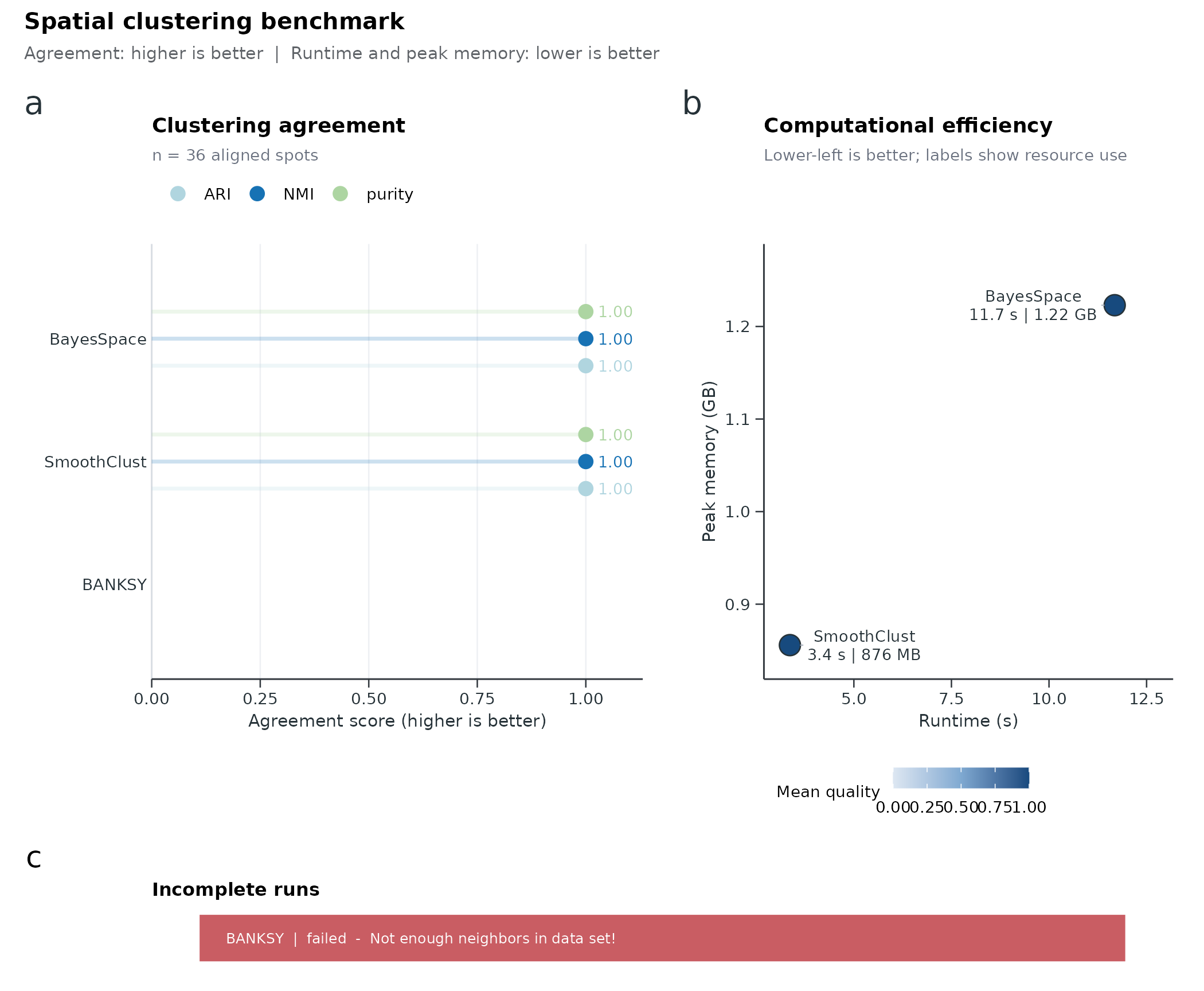
Other views:
SpatialBenchmarkPlot(data = bench, plot_type = "quality")
SpatialBenchmarkPlot(data = bench, plot_type = "efficiency")
SpatialBenchmarkPlot(data = bench, plot_type = "heatmap")
SpatialBenchmarkPlot(data = bench, plot_type = "funkyheatmap")
funkyheatmap is an explicit optional view. If its
dependency is unavailable, the call reports that availability condition;
it is never selected implicitly by auto.
What to report
A spatial benchmark report should include:
- the gold-standard column and number of domains;
- methods compared and any
method_paramsoverrides; -
$summarywith ARI, NMI, purity, runtime, and peak memory; - the overview or quality plot;
- failed or unavailable methods (status column) when backends are missing.
Agreement metrics are higher when better; runtime and peak memory are lower when better.