Integration benchmark workflow • scop

What you will do

Question: which method balances batch mixing and biological preservation on these cells?
Input: All 1,600 cells in panc8_sub, with tech for batch and celltype for biological evaluation.
Output: Per-method run status, latent-space metrics, summary plots and exported score tables.
How to run: start a fresh R session and run the chunks in order. Printed tables and figures below are generated from that run; code-only alternatives are identified explicitly.

This article compares batch-correction methods on the same scRNA-seq object with [RunIntegrationBenchmark()]. The runner scores each latent embedding (not UMAP) with scIB-style metrics, stores tables in srt@tools$IntegrationBenchmark, and returns the Seurat object for plotting with [IntegrationBenchmarkPlot()].

Use this workflow when you need a reproducible side-by-side report for Uncorrected, Harmony, fastMNN, or other [RunIntegration()] methods on the same input.

Prepare the required Harmony source

SCOP’s RunHarmony2() checks the official GitHub package origin. A CRAN installation with the same package name does not satisfy that check and can trigger an installation attempt in the middle of an analysis. Install the exact source before starting this page, then restart R:

remotes::install_github(
  "immunogenomics/harmony@df19af23ae0639bd6ea2da63898f973f08c85862",
  upgrade = "never"
)

The tutorial’s dependency preflight is read-only. It fails with a clear setup requirement instead of allowing an implicit installation during fitting.

Load data

library(scop)
set.seed(11)
harmony_source <- utils::packageDescription("harmony")
stopifnot(identical(harmony_source$RemoteUsername, "immunogenomics"),
          identical(harmony_source$RemoteSha, "df19af23ae0639bd6ea2da63898f973f08c85862"))
data.frame(package = "harmony", version = harmony_source$Version,
           source = paste(harmony_source$RemoteUsername, harmony_source$RemoteRepo, sep = "/"),
           revision = harmony_source$RemoteSha)
#>   package version                 source
#> 1 harmony   2.0.4 immunogenomics/harmony
#>                                   revision
#> 1 df19af23ae0639bd6ea2da63898f973f08c85862

data(panc8_sub)
table(panc8_sub$tech)
#> 
#>     celseq    celseq2 fluidigmc1     indrop  smartseq2 
#>        200        200        200        800        200
table(panc8_sub$celltype)
#> 
#>             acinar activated-stellate              alpha               beta 
#>                164                 50                483                428 
#>              delta             ductal        endothelial            epsilon 
#>                111                237                 26                  3 
#>              gamma         macrophage               mast quiescent-stellate 
#>                 67                  9                  7                 14 
#>            schwann 
#>                  1

Run the benchmark

Keep the batch column (tech) and a biological label column (celltype) fixed across methods. LISI and clustering metrics are computed on each method’s latent reduction (for example Harmony or Uncorrectedpca).

panc8_sub <- RunIntegrationBenchmark(
  panc8_sub,
  batch = "tech",
  celltype = "celltype",
  methods = c("Uncorrected", "Harmony"),
  nHVF = 2000,
  linear_reduction_dims = 50,
  linear_reduction_dims_use = 1:30,
  perplexity = 30,
  skip_failed = FALSE,
  nonlinear_reduction_dims = 2, seed = 11,
  verbose = FALSE
)
#> Warning: Data 1/5 of the `srt_list` is "unknown"
#> Warning: Data 2/5 of the `srt_list` is "unknown"
#> Warning: Data 3/5 of the `srt_list` is "unknown"
#> Warning: Data 4/5 of the `srt_list` is "unknown"
#> Warning: Data 5/5 of the `srt_list` is "unknown"
#> Warning: No layers found matching search pattern provided
#> Warning: Layer 'scale.data' is empty
#> Warning: No layers found matching search pattern provided
#> Warning: Layer 'scale.data' is empty

The 2,000 variable genes and 30 latent dimensions define the shared model input; all cells are scored. No cell subsampling is performed. skip_failed = FALSE stops this two-method comparison if either method fails, so one successful method cannot be mistaken for a complete comparison.

Print summary tables

Use thisplot::print_colored_table() on the stored tables. The summary view shows scaled overall, bio, and batch scores; the metrics view lists every metric per method.

bench <- panc8_sub@tools$IntegrationBenchmark
bench$runs
#>        method  status error runtime_s         latent              umap
#> 1 Uncorrected success          16.789 Uncorrectedpca UncorrectedUMAP2D
#> 2     Harmony success          11.610        Harmony     HarmonyUMAP2D
stopifnot(all(bench$runs$status == "success"))

thisplot::print_colored_table(
  bench$summary,
  by = "row",
  palette = "Chinese"
)
#> method       status   overall    bio        batch      iLISI      cLISI      celltype_ASW  batch_ASW_mixing  celltype_graph_connectivity  celltype_ARI  celltype_NMI  runtime_s  latent          umap             
#> Uncorrected  success  0.6753851  0.7860799  0.5093428  0.0632008  0.9892034  0.5881147     0.9554849         0.9713626                    0.4699072     0.7378917     16.789     Uncorrectedpca  UncorrectedUMAP2D
#> Harmony      success  0.7792839  0.8673961  0.6471157  0.3724491  0.9939972  0.6688506     0.9217823         0.9457216                    0.7628313     0.8654756     11.610     Harmony         HarmonyUMAP2D    

metrics <- bench$metrics
metrics <- metrics[
  !grepl("_LISI_mean$", metrics$metric), ,
  drop = FALSE
]
thisplot::print_colored_table(
  metrics,
  by = "col",
  palette = "Paired"
)
#> metric                       category  value      scaled     direction  method     
#> batch_ASW_mixing             batch     0.9554849  0.9554849  higher     Uncorrected
#> celltype_ASW                 bio       0.1762294  0.5881147  higher     Uncorrected
#> celltype_graph_connectivity  bio       0.9713626  0.9713626  higher     Uncorrected
#> celltype_NMI                 bio       0.7378917  0.7378917  higher     Uncorrected
#> celltype_ARI                 bio       0.4699072  0.4699072  higher     Uncorrected
#> celltype_purity              bio       0.9600000  0.9600000  higher     Uncorrected
#> iLISI                        batch     1.2528032  0.0632008  higher     Uncorrected
#> cLISI                        bio       1.1295592  0.9892034  higher     Uncorrected
#> batch_ASW_mixing             batch     0.9217823  0.9217823  higher     Harmony    
#> celltype_ASW                 bio       0.3377013  0.6688506  higher     Harmony    
#> celltype_graph_connectivity  bio       0.9457216  0.9457216  higher     Harmony    
#> celltype_NMI                 bio       0.8654756  0.8654756  higher     Harmony    
#> celltype_ARI                 bio       0.7628313  0.7628313  higher     Harmony    
#> celltype_purity              bio       0.9675000  0.9675000  higher     Harmony    
#> iLISI                        batch     2.4897966  0.3724491  higher     Harmony    
#> cLISI                        bio       1.0720339  0.9939972  higher     Harmony

Read the scores without overclaiming

Read the value and scaled columns separately. Raw iLISI increases when neighborhoods contain more batches; raw cLISI is closest to 1 when a neighborhood retains a single cell type. The scaled cLISI score reverses that direction so larger scaled values represent better label preservation. The printed direction field refers to the scaled score, not raw cLISI.

The biological summary combines label separation, connectivity and clustering agreement. The batch summary combines mixing measures. The overall score uses 60% biological and 40% batch weight by default; it is a chosen trade-off, not a probability of success. Inspect every metric and the label-by-batch balance before preferring a method. A high batch score can accompany overcorrection, and labels unique to one technology cannot be made to mix legitimately.

Missing metrics remain missing rather than becoming a successful result. This small bundled study subset illustrates comparison on the same cells; it does not establish a universal ranking of integration methods. To adapt the benchmark, keep input cells, feature selection, dimensions and evaluation labels fixed, then report the same raw tables and run statuses for each method.

Plot all views

IntegrationBenchmarkPlot() with plot_type = "auto" returns a named list: box (per-cell LISI), heatmap, scatter, and umap.

plots <- IntegrationBenchmarkPlot(panc8_sub, verbose = FALSE)
names(plots)
#> [1] "box"     "heatmap" "scatter" "umap"
plots$box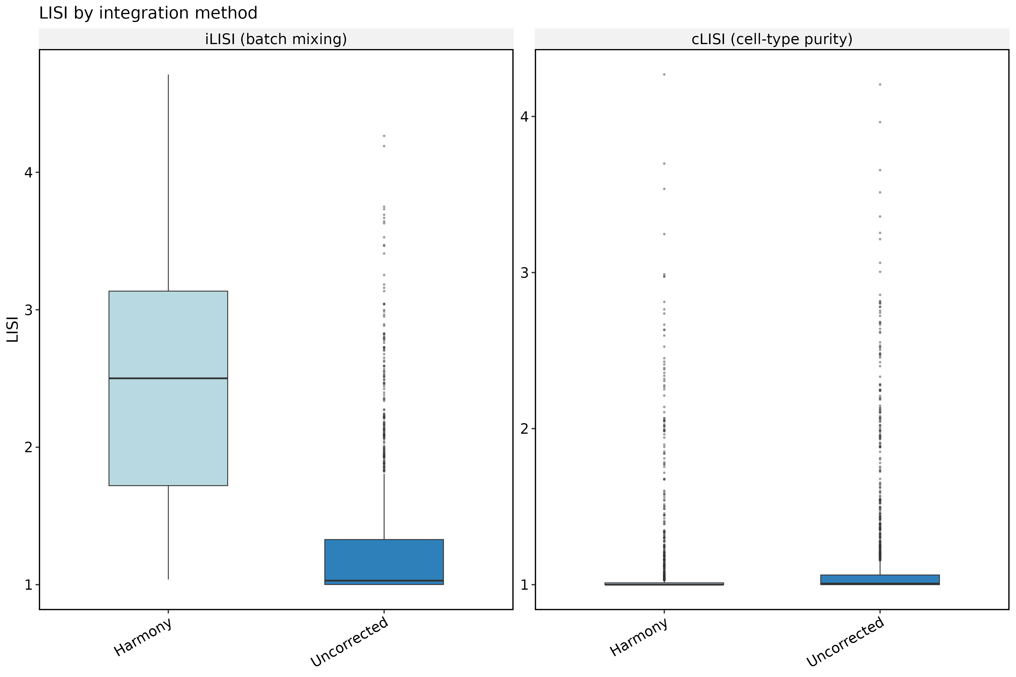

plots$scatter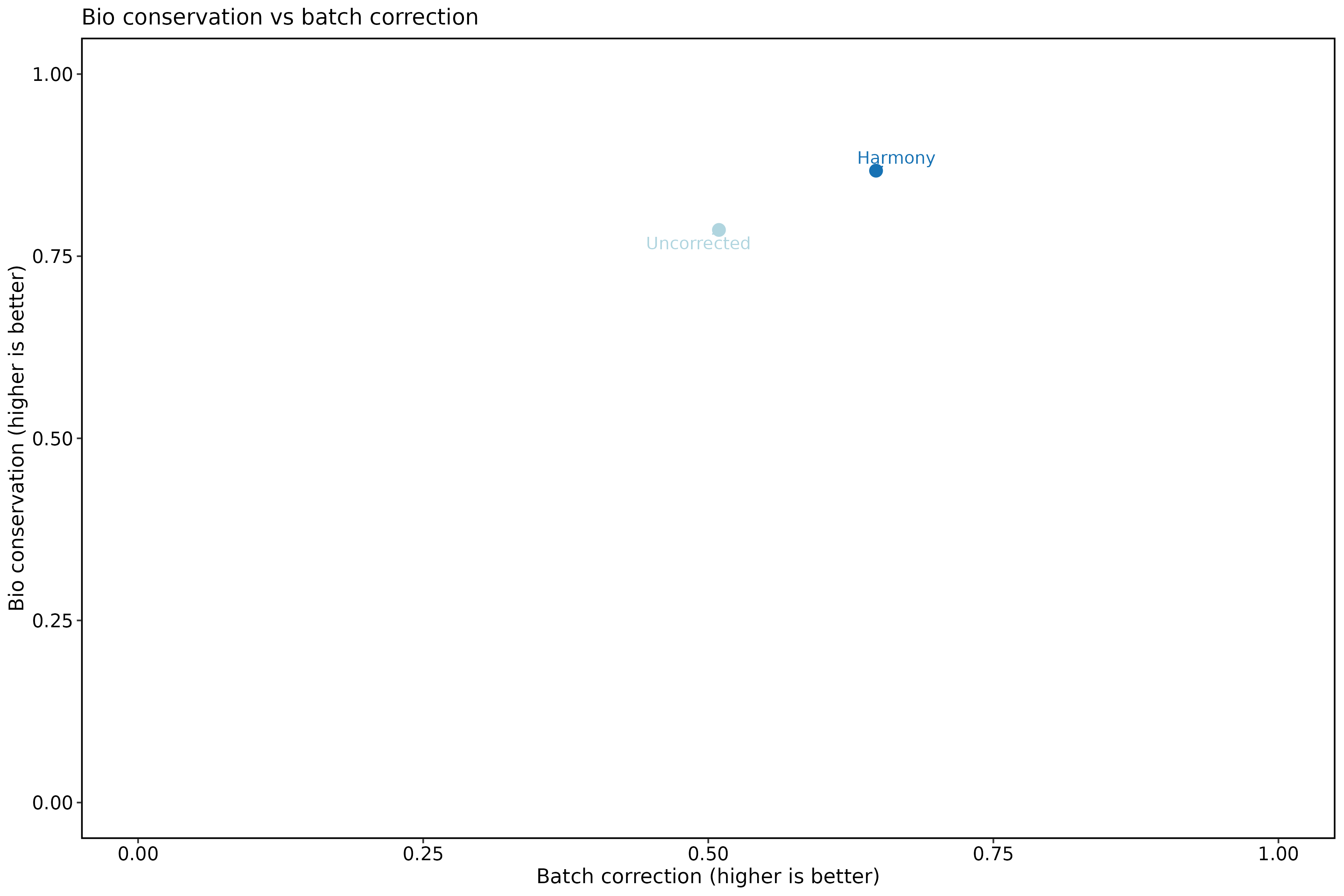

plots$heatmap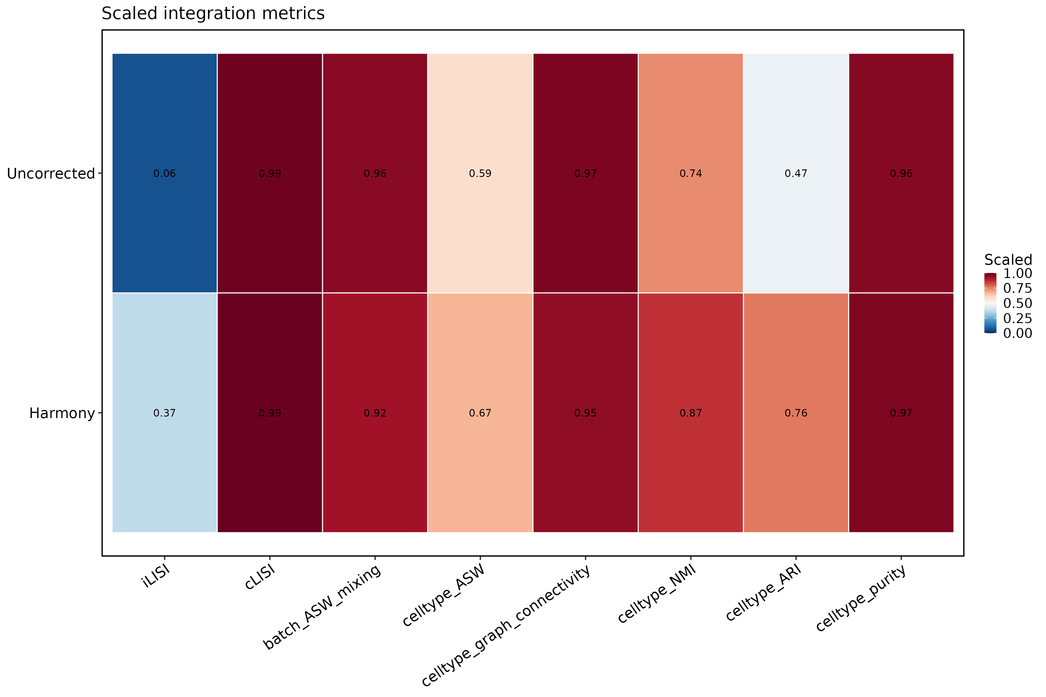

plots$umap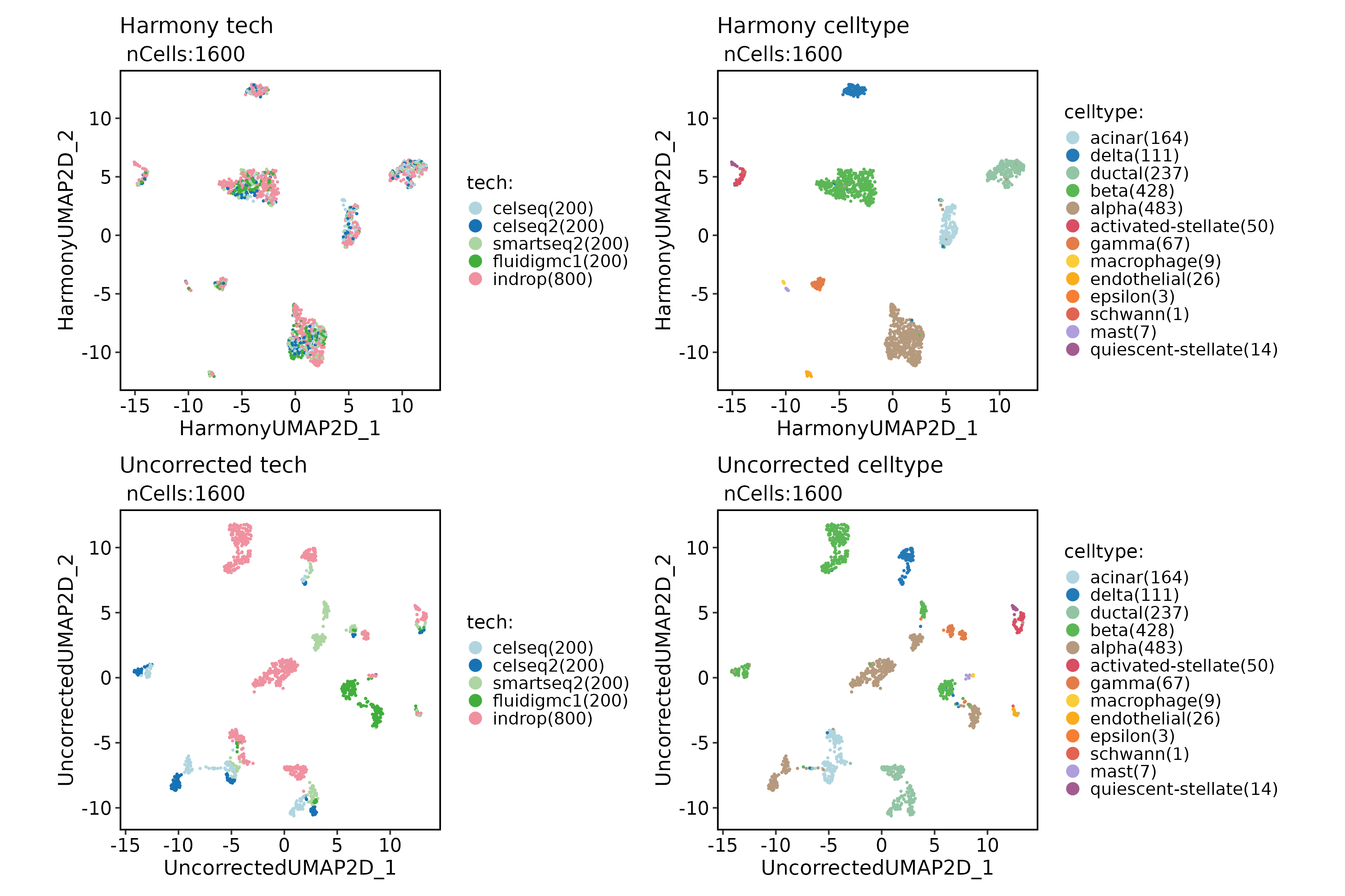

Individual plot types are also available:

IntegrationBenchmarkPlot(panc8_sub, plot_type = "box")
IntegrationBenchmarkPlot(panc8_sub, plot_type = "umap")

Save, reload, and check the hand-off

The build uses a temporary directory so repeated rendering cannot overwrite a previous analysis. For your work, replace it with a new persistent output folder. Save the object and plain-text metadata; a figure alone cannot reproduce the analysis. No cells are sampled for this export.

output_dir <- file.path(tempdir(), "integration-benchmark-workflow")
dir.create(output_dir, recursive = TRUE, showWarnings = FALSE)
result_file <- file.path(output_dir, "analysis.rds")
saveRDS(panc8_sub, result_file)
utils::write.csv(bench$summary, file.path(output_dir, "benchmark-summary.csv"), row.names = FALSE)
utils::write.csv(bench$metrics, file.path(output_dir, "benchmark-metrics.csv"), row.names = FALSE)
utils::write.csv(bench$runs, file.path(output_dir, "benchmark-runs.csv"), row.names = FALSE)
utils::write.csv(panc8_sub@meta.data, file.path(output_dir, "cell-metadata.csv"))
reloaded <- readRDS(result_file)
stopifnot(identical(colnames(reloaded), colnames(panc8_sub)),
          identical(reloaded@meta.data, panc8_sub@meta.data),
          identical(SeuratObject::Reductions(reloaded),
                    SeuratObject::Reductions(panc8_sub)))
data.frame(file = basename(list.files(output_dir, full.names = TRUE)),
           bytes = file.info(list.files(output_dir, full.names = TRUE))$size)
#>                    file    bytes
#> 1          analysis.rds 41787713
#> 2 benchmark-metrics.csv     1601
#> 3    benchmark-runs.csv      180
#> 4 benchmark-summary.csv      657
#> 5     cell-metadata.csv   274267

Use your own data and recover common errors

Replace the data(...) input with readRDS("your-object.rds"), or create a Seurat object from a gene-by-cell raw-count matrix. Check that cell IDs are unique and metadata row names equal the expression column names.
Set the assay and grouping columns explicitly. Species, gene identifiers and reference labels must match your experiment; do not copy pancreas labels to unrelated tissue.
If a reduction or metadata column is missing, inspect SeuratObject::Reductions(object) and colnames(object@meta.data), then run its producer chunk. A plot does not create the result it needs.
If a dependency is unavailable, install it in the analysis environment, restart R and rerun from the input chunk. A skipped or failed method is not evidence that it worked. Preserve warnings and the exact error in your report.

Build and analysis provenance

The receipt records the R seed. Python methods retain their documented backend seeds and parameters; setting the R seed alone does not control every backend. Package versions, BLAS libraries and backend changes can alter numerical results. Keep this receipt with the exported object. It describes this page’s actual render.

source_revision <- Sys.getenv("GITHUB_SHA")
if (!nzchar(source_revision) && nzchar(Sys.which("git"))) {
  source_revision <- tryCatch(system2("git", c("rev-parse", "HEAD"), stdout = TRUE,
                                      stderr = FALSE)[1], error = function(e) NA_character_)
}
article_source <- knitr::current_input(dir = TRUE)
build_receipt <- data.frame(
  article = "integration-benchmark-workflow",
  built_utc = format(Sys.time(), tz = "UTC", usetz = TRUE),
  scop = as.character(utils::packageVersion("scop")),
  R = as.character(getRversion()),
  source_revision = source_revision,
  source_has_local_changes = if (nzchar(Sys.which("git")))
    length(system2("git", c("status", "--porcelain"), stdout = TRUE, stderr = FALSE)) > 0 else NA,
  article_md5 = unname(tools::md5sum(article_source)),
  R_seed = 11,
  cells_retained = ncol(panc8_sub),
  genes_in_active_assay = nrow(panc8_sub),
  stringsAsFactors = FALSE
)
build_receipt
#>                          article               built_utc  scop     R
#> 1 integration-benchmark-workflow 2026-10-12 00:07:23 UTC 0.9.2 4.6.1
#>                            source_revision source_has_local_changes
#> 1 083f5f31e37220a9e9a5b0110e63ea4ed3f49317                    FALSE
#>                        article_md5 R_seed cells_retained genes_in_active_assay
#> 1 d71cb1f95a7667cb9b3dfc8e9fce882a     11           1600                 12932
utils::write.csv(build_receipt, file.path(output_dir, "build-receipt.csv"),
                 row.names = FALSE)
writeLines(capture.output(sessionInfo()), file.path(output_dir, "session-info.txt"))

Show the complete R session used for this page

sessionInfo()
#> R version 4.6.1 (2026-06-24)
#> Platform: x86_64-pc-linux-gnu
#> Running under: Ubuntu 24.04.5 LTS
#> 
#> Matrix products: default
#> BLAS:   /usr/lib/x86_64-linux-gnu/openblas-pthread/libblas.so.3 
#> LAPACK: /usr/lib/x86_64-linux-gnu/openblas-pthread/libopenblasp-r0.3.26.so;  LAPACK version 3.12.0
#> 
#> locale:
#>  [1] LC_CTYPE=C.UTF-8       LC_NUMERIC=C           LC_TIME=C.UTF-8       
#>  [4] LC_COLLATE=C.UTF-8     LC_MONETARY=C.UTF-8    LC_MESSAGES=C.UTF-8   
#>  [7] LC_PAPER=C.UTF-8       LC_NAME=C              LC_ADDRESS=C          
#> [10] LC_TELEPHONE=C         LC_MEASUREMENT=C.UTF-8 LC_IDENTIFICATION=C   
#> 
#> time zone: UTC
#> tzcode source: system (glibc)
#> 
#> attached base packages:
#> [1] stats     graphics  grDevices utils     datasets  methods   base     
#> 
#> other attached packages:
#> [1] scop_0.9.2
#> 
#> loaded via a namespace (and not attached):
#>   [1] RColorBrewer_1.1-3       jsonlite_2.0.0           shape_1.4.6.1           
#>   [4] magrittr_2.0.5           spatstat.utils_3.2-5     farver_2.1.2            
#>   [7] rmarkdown_2.32           GlobalOptions_0.1.4      fs_2.1.0                
#>  [10] ragg_1.5.2               vctrs_0.7.3              ROCR_1.0-12             
#>  [13] Rsamtools_2.28.0         spatstat.explore_3.8-3   RcppRoll_0.4.0          
#>  [16] htmltools_0.5.9          BiocNeighbors_2.6.0      sass_0.4.10             
#>  [19] thisutils_0.5.2          sctransform_0.4.3        parallelly_1.48.0       
#>  [22] KernSmooth_2.23-26       bslib_0.12.0             htmlwidgets_1.6.4       
#>  [25] desc_1.4.3               ica_1.0-3                plyr_1.8.9              
#>  [28] plotly_4.12.1            zoo_1.9-1                cachem_1.1.0            
#>  [31] igraph_2.3.4             mime_0.13                lifecycle_1.0.5         
#>  [34] iterators_1.0.14         pkgconfig_2.0.3          Matrix_1.7-5            
#>  [37] R6_2.6.1                 fastmap_1.2.0            MatrixGenerics_1.24.0   
#>  [40] fitdistrplus_1.2-6       future_1.76.0            shiny_1.14.0            
#>  [43] clue_0.3-68              digest_0.6.39            thisplot_0.4.6          
#>  [46] colorspace_2.1-4         patchwork_1.3.2          S4Vectors_0.50.3        
#>  [49] Seurat_5.6.0             tensor_1.5.1             RSpectra_0.16-2         
#>  [52] irlba_2.4.1              GenomicRanges_1.64.0     textshaping_1.0.5       
#>  [55] labeling_0.4.3           progressr_1.0.0          spatstat.sparse_3.2-0   
#>  [58] httr_1.4.9               polyclip_1.10-7          abind_1.4-8             
#>  [61] compiler_4.6.1           withr_3.0.3              doParallel_1.0.17       
#>  [64] S7_0.2.2                 BiocParallel_1.46.0      fastDummies_1.7.6       
#>  [67] ggforce_0.5.0            MASS_7.3-65              proxyC_0.5.2            
#>  [70] rjson_0.2.23             tools_4.6.1              lmtest_0.9-40           
#>  [73] otel_0.2.0               httpuv_1.6.17            future.apply_1.20.2     
#>  [76] goftest_1.2-3            glue_1.8.1               nlme_3.1-169            
#>  [79] promises_1.5.0           grid_4.6.1               Rtsne_0.17              
#>  [82] cluster_2.1.8.2          reshape2_1.4.5           generics_0.1.4          
#>  [85] gtable_0.3.6             spatstat.data_3.1-9      tidyr_1.3.2             
#>  [88] data.table_1.18.6.1      XVector_0.52.0           sp_2.2-3                
#>  [91] BiocGenerics_0.58.1      spatstat.geom_3.8-3      RcppAnnoy_0.0.23        
#>  [94] ggrepel_0.9.8            RANN_2.6.3               foreach_1.5.2           
#>  [97] pillar_1.11.1            stringr_1.6.0            spam_2.11-4             
#> [100] RcppHNSW_0.7.0           later_1.4.8              circlize_0.4.18         
#> [103] splines_4.6.1            tweenr_2.0.3             dplyr_1.2.1             
#> [106] lattice_0.22-9           survival_3.8-6           deldir_2.0-4            
#> [109] tidyselect_1.2.1         ComplexHeatmap_2.28.0    Biostrings_2.80.2       
#> [112] miniUI_0.1.2             pbapply_1.7-5            knitr_1.52              
#> [115] gridExtra_2.3.1          Seqinfo_1.2.0            IRanges_2.46.0          
#> [118] scattermore_1.2          RhpcBLASctl_0.23-42      stats4_4.6.1            
#> [121] xfun_0.61                matrixStats_1.5.0        UCSC.utils_1.8.0        
#> [124] stringi_1.8.9            yaml_2.3.12              evaluate_1.0.5          
#> [127] codetools_0.2-20         tibble_3.3.1             cli_3.6.6               
#> [130] uwot_0.2.5               RcppParallel_6.2.1       Signac_1.17.1           
#> [133] xtable_1.8-8             reticulate_1.47.0        systemfonts_1.3.2       
#> [136] jquerylib_0.1.4          harmony_2.0.4            GenomeInfoDb_1.48.0     
#> [139] dichromat_2.0-1          Rcpp_1.1.2               spatstat.random_3.5-2   
#> [142] globals_0.19.1           png_0.1-9                spatstat.univar_3.2-0   
#> [145] parallel_4.6.1           pkgdown_2.2.1            ggplot2_4.0.3           
#> [148] dotCall64_1.2            sparseMatrixStats_1.24.0 bitops_1.1-0            
#> [151] listenv_1.1.0            viridisLite_0.4.3        scales_1.4.0            
#> [154] ggridges_0.5.7           SeuratObject_5.4.0       purrr_1.2.2             
#> [157] crayon_1.5.3             GetoptLong_1.1.1         rlang_1.3.0             
#> [160] fastmatch_1.1-8          cowplot_1.2.0

What to report

A compact integration benchmark report should include:

batch and cell-type columns used for scoring;
methods compared and shared integration parameters (nHVF, latent dimensions);
the colored summary and metrics tables;
LISI boxplots, bio-vs-batch scatter, and UMAP panels colored by batch and cell type.

Overall score uses scIB weights: 0.6 * bio + 0.4 * batch. Higher is better for all scaled metrics shown in the summary table.

A higher batch score alone can reward overcorrection. Compare biological retention, batch mixing and marker patterns together. Results depend on this dataset and labels, and do not establish a universally best integration method.