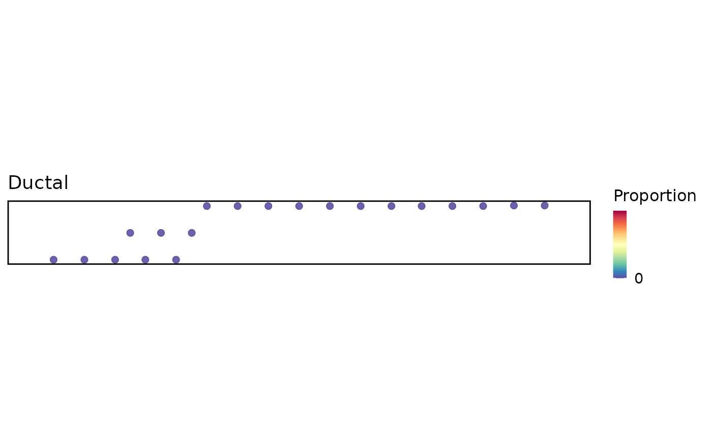
Plot stored spatial deconvolution proportions

Plot spot-by-cell-type proportions stored by RunRCTD(), RunCARD(), RunSPOTlight(). The plot reads the stored result directly from srt@tools[[tool_name]] and never reruns a deconvolution backend. RunCSIDE() is intentionally excluded because its output represents differential or context effects rather than cell-type proportions.

Usage

SpatialDeconvolutionPlot(
  object,
  tool_name = NULL,
  cell_types = NULL,
  plot_type = c("point", "dominant", "pie"),
  combine = TRUE,
  nrow = NULL,
  ncol = NULL,
  byrow = TRUE,
  ...,
  image.scale = c("lowres", "hires"),
  srt = NULL
)

Arguments

object

A spatial Seurat object containing a stored deconvolution result.

tool_name

Explicit non-empty key in srt@tools. Results are never discovered implicitly.

cell_types

Optional cell types to display. The default uses all stored cell types.

plot_type

Plot proportions as separate point maps, one dominant-type map derived from the stored proportions, or one spot-level pie map.

combine

Whether to combine point or dominant maps. If FALSE, return a named list.

nrow, ncol, byrow

Point-map layout controls. When both dimensions are NULL, a near-square layout with at most three columns is used.

...

Additional arguments passed to SpatialSpotPlot().

image.scale

Image scale factor matching the selected raster.

srt

Deprecated alias for object; supply exactly one of the two. It will be removed in scop 1.0.0.

Value

A ggplot, patchwork, or named list of ggplot objects.

Details

Point maps share a zero-to-one scale. A cell type with no measured values produces an informative empty panel instead of aborting the other maps. For dominant and pie maps, cell_types selects the types participating in the displayed comparison; pie fractions are relative to those selected types.

Examples

data(visium_human_pancreas_sub)
data(panc8_sub)
reference <- panc8_sub[, panc8_sub$celltype %in% c("ductal", "alpha", "beta")]
reference <- Seurat::FindVariableFeatures(reference, nfeatures = 300, verbose = FALSE)
features <- head(intersect(
  SeuratObject::VariableFeatures(reference),
  rownames(visium_human_pancreas_sub)
), 300)
spatial <- RunRCTD(
  visium_human_pancreas_sub,
  reference = reference,
  reference_label = "celltype",
  features = features,
  assay = "Spatial",
  reference_assay = "RNA",
  layer = "counts",
  reference_layer = "counts",
  rctd_mode = "full",
  max_cores = 1,
  verbose = FALSE
)
#> Begin: process_cell_type_info
#> process_cell_type_info: number of cells in reference: 1148
#> process_cell_type_info: number of genes in reference: 97
#> 
#> ductal   beta  alpha 
#>    237    428    483 
#> End: process_cell_type_info
#> create.RCTD: getting regression differentially expressed genes: 
#> get_de_genes: ductal found DE genes: 22
#> get_de_genes: beta found DE genes: 4
#> get_de_genes: alpha found DE genes: 1
#> get_de_genes: total DE genes: 27
#> create.RCTD: getting platform effect normalization differentially expressed genes: 
#> get_de_genes: ductal found DE genes: 26
#> get_de_genes: beta found DE genes: 7
#> get_de_genes: alpha found DE genes: 2
#> get_de_genes: total DE genes: 35
#> fitBulk: decomposing bulk
#> chooseSigma: using initial Q_mat with sigma =  1
#> Likelihood value: 40089.2008086036
#> Sigma value:  0.84
#> Likelihood value: 39342.4105815425
#> Sigma value:  0.69
#> Likelihood value: 38786.8209416109
#> Sigma value:  0.61
#> Likelihood value: 38578.9034272757
#> Sigma value:  0.53
#> Likelihood value: 38653.2368763574
#> Sigma value:  0.49
#> Likelihood value: 38432.7589536896
#> Sigma value:  0.48
#> Likelihood value: 38431.5741354963
#> Sigma value:  0.48
SpatialDeconvolutionPlot(spatial, tool_name = "RCTD", plot_type = "dominant")