Cell-cell communication workflow • scop

This article shows a practical first-pass workflow for cell-cell communication analysis in scop: prepare a cell-type annotation, run ligand-receptor inference, inspect sender-receiver summaries, then focus on specific ligands, receptors, pathways, or downstream targets only after the global result looks stable.

This workflow starts from single-cell expression data. For spatially constrained communication, use RunSpatialCellChat() and the spatial workflow article. SpatialCellChat is stored as a distinct CCC method because its distance constraint and spatial permutation basis are not interchangeable with non-spatial CellChat scores.

The examples below use the bundled pancreas_sub data and run the R-side CellChat and LIANA wrappers directly when those optional packages are available. CellphoneDB is intentionally not used here because it requires a Python environment and a CellPhoneDB database.

scop keeps the workflow unified in three layers:

Layer	Entry point	Purpose
Result tables	`RunCCC()` output	Store standardized `long_table`, `pair_table`, and method status in `srt@tools$CCC`.
Heatmap layer	`CCCHeatmap()`	Matrix, dot, tile, sample, pathway, and differential heatmap views.
Statistical layer	`CCCStatPlot()`	Ranked interactions, distributions, pathway summaries, and comparison statistics.
Network layer	`CCCNetworkPlot()`	Sender-receiver networks, pathway networks, embedding networks, and focused ligand-receptor flow.

The plots in this article summarize inferred ligand-receptor evidence. A high score means the selected method found strong expression-based support for a sender ligand, receiver receptor, and sender-receiver context. It should not be read as a direct measurement of secreted protein amount, physical distance, or causal signaling.

Prepare the Object

Start with a normalized Seurat object and a metadata column that represents the cell identities used as sender and receiver groups. For the bundled pancreas example, CellType is the coarse annotation and SubCellType is the finer annotation.

library(scop)
#>           ⬢          .        ⬡             ⬢     .
#>                      _____ _________  ____
#>                     / ___// ___/ __ ./ __ .
#>                    (__  )/ /__/ /_/ / /_/ /
#>                   /____/ .___/.____/ .___/
#>                                   /_/
#>       ⬢               .      ⬡        .          ⬢
#> ------------------------------------------------------------
#> Version: 0.8.9 (2026-07-20 update)
#> Website: https://mengxu98.github.io/scop/
#> 
#> Python environment initialization is disabled
#> To enable it, set: options(scop_env_init = TRUE)
#> 
#> The message can be suppressed by: 
#>   suppressPackageStartupMessages(library(scop))
#>   or options(log_message.verbose = FALSE)
#> ------------------------------------------------------------
library(ggplot2)

data(pancreas_sub)
pancreas_sub <- standard_scop(pancreas_sub, verbose = FALSE)
#> ℹ [2026-07-28 03:36:23] Skip `log1p()` because `layer = data` is not "counts"

table(pancreas_sub$CellType)
#> 
#>        Ductal     Endocrine  Ngn3-high-EP   Ngn3-low-EP Pre-endocrine 
#>           253           355           169            67           156
table(pancreas_sub$SubCellType)
#> 
#>         Alpha          Beta         Delta        Ductal       Epsilon 
#>           121           174            20           253            40 
#>  Ngn3-high-EP   Ngn3-low-EP Pre-endocrine 
#>           169            67           156

Use the same visual settings across the article so that heatmaps, statistical summaries, and network plots can be compared without changing palettes or text scale.

ccc_cell_pal <- c(
  "Ductal" = "#4E79A7",
  "Endocrine" = "#E15759",
  "Ngn3-high-EP" = "#59A14F",
  "Ngn3-low-EP" = "#76B7B2",
  "Pre-endocrine" = "#F28E2B"
)

ccc_value_pal <- c("#2C5C85", "#8FBBD9", "#F7F7F7", "#F2B38F", "#B9473D")

ccc_theme_args <- list(base_size = 11)

Before communication analysis, check whether groups have enough cells or whether some labels should be merged. CCC methods compare group-level expression, so unstable labels usually become noisy sender-receiver edges. The bundled pancreas_sub object is used as-is in this article.

cell_counts <- sort(table(pancreas_sub$CellType), decreasing = TRUE)
cell_counts
#> 
#>     Endocrine        Ductal  Ngn3-high-EP Pre-endocrine   Ngn3-low-EP 
#>           355           253           169           156            67

pancreas_ccc <- pancreas_sub
pancreas_ccc$CellType <- droplevels(factor(pancreas_ccc$CellType))

table(pancreas_ccc$CellType)
#> 
#>        Ductal     Endocrine  Ngn3-high-EP   Ngn3-low-EP Pre-endocrine 
#>           253           355           169            67           156

Run a CCC Screen

RunCCC() is the shortest path when the goal is to compare the same object with several ligand-receptor scoring methods. In this article, it runs CellChat and LIANA when both optional R backends are installed, then rebuilds the unified srt@tools$CCC tables for common downstream plots.

pancreas_ccc <- RunCCC(
  pancreas_ccc,
  group.by = "CellType",
  methods = c("CellChat", "LIANA"),
  method_params = list(
    CellChat = list(species = "Mus_musculus", min.cells = 5),
    LIANA = list(
      method = c("natmi", "connectome"),
      resource = "Consensus",
      min_cells = 5
    )
  ),
  skip_failed = TRUE,
  thresh = 0.05,
  verbose = FALSE
)
#> [1] "Create a CellChat object from a data matrix"
#> Set cell identities for the new CellChat object 
#> The cell groups used for CellChat analysis are  Ductal, Endocrine, Ngn3-high-EP, Ngn3-low-EP, Pre-endocrine 
#> The number of highly variable ligand-receptor pairs used for signaling inference is 841 
#> triMean is used for calculating the average gene expression per cell group. 
#> [1] ">>> Run CellChat on sc/snRNA-seq data <<< [2026-07-28 03:36:37.451636]"
#> [1] ">>> CellChat inference is done. Parameter values are stored in `object@options$parameter` <<< [2026-07-28 03:37:11.739716]"
#> Warning: `invoke()` is deprecated as of rlang 0.4.0.
#> Please use `exec()` or `inject()` instead.
#> This warning is displayed once every 8 hours.
#> Warning in .local(x, ...): 'librarySizeFactors' is deprecated.
#> Use 'scrapper::centerSizeFactors' instead.
#> See help("Deprecated")
#> Warning in .local(x, ...): 'librarySizeFactors' is deprecated.
#> Use 'scrapper::centerSizeFactors' instead.
#> See help("Deprecated")
#> Warning in .local(x, ...): 'librarySizeFactors' is deprecated.
#> Use 'scrapper::centerSizeFactors' instead.
#> See help("Deprecated")
#> Warning in .local(x, ...): 'librarySizeFactors' is deprecated.
#> Use 'scrapper::centerSizeFactors' instead.
#> See help("Deprecated")
#> Warning in .local(x, ...): 'librarySizeFactors' is deprecated.
#> Use 'scrapper::centerSizeFactors' instead.
#> See help("Deprecated")
#> Warning in .local(x, ...): 'librarySizeFactors' is deprecated.
#> Use 'scrapper::centerSizeFactors' instead.
#> See help("Deprecated")
#> Warning in .local(x, ...): 'librarySizeFactors' is deprecated.
#> Use 'scrapper::centerSizeFactors' instead.
#> See help("Deprecated")
#> Warning in .local(x, ...): 'librarySizeFactors' is deprecated.
#> Use 'scrapper::centerSizeFactors' instead.
#> See help("Deprecated")
#> Warning in .local(x, ...): 'librarySizeFactors' is deprecated.
#> Use 'scrapper::centerSizeFactors' instead.
#> See help("Deprecated")
#> Warning in .local(x, ...): 'librarySizeFactors' is deprecated.
#> Use 'scrapper::centerSizeFactors' instead.
#> See help("Deprecated")
#> Warning in .summarize_assay_by_group(assay(x, assay.type), ...): 'summarizeAssayByGroup' is deprecated.
#> Use 'scrapper::aggregateAcrossCells' or 'beachmat::tatami.sums.by.group' instead.
#> Warning in .summarize_assay_by_group(assay(x, assay.type), ...): 'summarizeAssayByGroup' is deprecated.
#> Use 'scrapper::aggregateAcrossCells' or 'beachmat::tatami.sums.by.group' instead.
#> Warning in .findMarkers(assay(x, i = assay.type), ...): 'findMarkers' is deprecated.
#> Use 'scrapper::scoreMarkers.se' instead.
#> See help("Deprecated")
#> Warning in .local(x, ...): 'pairwiseWilcox' is deprecated.
#> See help("Deprecated")
#> Warning in combineMarkers(fit$statistics, fit$pairs, pval.type = pval.type, : 'combineMarkers' is deprecated.
#> Use 'scrapper::summarizeEffects' instead.
#> See help("Deprecated")
#> Warning: There were 2 warnings in `mutate()`.
#> The first warning was:
#> ℹ In argument: `ligand.prop = min(ligand.prop)`.
#> Caused by warning in `min()`:
#> ! no non-missing arguments to min; returning Inf
#> ℹ Run `dplyr::last_dplyr_warnings()` to see the 1 remaining warning.
#> Warning: There was 1 warning in `mutate()`.
#> ℹ In argument: `ligand.expr.min = min(.data[["ligand.expr"]])`.
#> Caused by warning in `min()`:
#> ! no non-missing arguments to min; returning Inf
#> Warning: There was 1 warning in `mutate()`.
#> ℹ In argument: `receptor.expr.min = min(.data[["receptor.expr"]])`.
#> Caused by warning in `min()`:
#> ! no non-missing arguments to min; returning Inf
#> Warning: There were 2 warnings in `mutate()`.
#> The first warning was:
#> ℹ In argument: `ligand.prop = min(ligand.prop)`.
#> Caused by warning in `min()`:
#> ! no non-missing arguments to min; returning Inf
#> ℹ Run `dplyr::last_dplyr_warnings()` to see the 1 remaining warning.
#> Warning: There was 1 warning in `mutate()`.
#> ℹ In argument: `ligand.scaled.min = min(.data[["ligand.scaled"]])`.
#> Caused by warning in `min()`:
#> ! no non-missing arguments to min; returning Inf
#> Warning: There was 1 warning in `mutate()`.
#> ℹ In argument: `receptor.scaled.min = min(.data[["receptor.scaled"]])`.
#> Caused by warning in `min()`:
#> ! no non-missing arguments to min; returning Inf

Check the run status and standardized result tables before plotting. Use pancreas_ccc@tools$CCC$long_table for ligand-receptor questions and pancreas_ccc@tools$CCC$pair_table for sender-receiver summaries. The long table is the most detailed layer: one row per method-specific ligand-receptor sender-receiver event. The pair table aggregates those rows to cell-type pairs, so it is useful for overview plots but less useful for naming specific biology.

pancreas_ccc@tools$RunCCC$status
#>     method    status elapsed message
#> 1 CellChat completed  38.908    <NA>
#> 2    LIANA completed   5.739    <NA>
pancreas_ccc@tools$RunCCC$completed_methods
#> [1] "CellChat" "LIANA"

ccc_long <- pancreas_ccc@tools$CCC$long_table
ccc_pair <- pancreas_ccc@tools$CCC$pair_table

head(ccc_long)
#>        sender    receiver ligand      receptor        score pvalue
#> 1      Ductal Ngn3-low-EP   Bmp7 BMPR1A_ACVR2B 0.0013409975      0
#> 2 Ngn3-low-EP Ngn3-low-EP   Bmp7 BMPR1A_ACVR2B 0.0010170280      0
#> 3      Ductal Ngn3-low-EP  Wnt7b     FZD2_LRP6 0.0010408195      0
#> 4 Ngn3-low-EP Ngn3-low-EP  Wnt7b     FZD2_LRP6 0.0009996108      0
#> 5      Ductal      Ductal   Igf2         Igf1r 0.0031658123      0
#> 6 Ngn3-low-EP      Ductal   Igf2         Igf1r 0.0036996124      0
#>     interaction_name      interaction_name_2 pathway_name         annotation
#> 1 BMP7_BMPR1A_ACVR2B Bmp7  - (Bmpr1a+Acvr2b)          BMP Secreted Signaling
#> 2 BMP7_BMPR1A_ACVR2B Bmp7  - (Bmpr1a+Acvr2b)          BMP Secreted Signaling
#> 3    WNT7B_FZD2_LRP6    Wnt7b  - (Fzd2+Lrp6)          WNT Secreted Signaling
#> 4    WNT7B_FZD2_LRP6    Wnt7b  - (Fzd2+Lrp6)          WNT Secreted Signaling
#> 5         IGF2_IGF1R           Igf2  - Igf1r          IGF Secreted Signaling
#> 6         IGF2_IGF1R           Igf2  - Igf1r          IGF Secreted Signaling
#>                         evidence dataset      interaction_label classification
#> 1  KEGG: mmu04350; PMID:26893264     ALL Bmp7 - (Bmpr1a+Acvr2b)            BMP
#> 2  KEGG: mmu04350; PMID:26893264     ALL Bmp7 - (Bmpr1a+Acvr2b)            BMP
#> 3 KEGG: mmu04310; PMID: 23209147     ALL    Wnt7b - (Fzd2+Lrp6)            WNT
#> 4 KEGG: mmu04310; PMID: 23209147     ALL    Wnt7b - (Fzd2+Lrp6)            WNT
#> 5                 PMID: 14604834     ALL           Igf2 - Igf1r            IGF
#> 6                 PMID: 14604834     ALL           Igf2 - Igf1r            IGF
#>                   pair_lr ligand_display receptor_display
#> 1 Bmp7  - (Bmpr1a+Acvr2b)           Bmp7    BMPR1A_ACVR2B
#> 2 Bmp7  - (Bmpr1a+Acvr2b)           Bmp7    BMPR1A_ACVR2B
#> 3    Wnt7b  - (Fzd2+Lrp6)          Wnt7b        FZD2_LRP6
#> 4    Wnt7b  - (Fzd2+Lrp6)          Wnt7b        FZD2_LRP6
#> 5           Igf2  - Igf1r           Igf2            Igf1r
#> 6           Igf2  - Igf1r           Igf2            Igf1r
#>      interaction_display significant neglog10_pvalue   method
#> 1 Bmp7 - (Bmpr1a+Acvr2b)        TRUE              NA CellChat
#> 2 Bmp7 - (Bmpr1a+Acvr2b)        TRUE              NA CellChat
#> 3    Wnt7b - (Fzd2+Lrp6)        TRUE              NA CellChat
#> 4    Wnt7b - (Fzd2+Lrp6)        TRUE              NA CellChat
#> 5           Igf2 - Igf1r        TRUE              NA CellChat
#> 6           Igf2 - Igf1r        TRUE              NA CellChat
head(ccc_pair)
#>      sender      receiver        sum        mean        max count
#> 1    Ductal        Ductal 0.90457295 0.026605087 0.21509356    34
#> 2    Ductal     Endocrine 0.30213984 0.037767480 0.22022319     8
#> 3    Ductal  Ngn3-high-EP 0.48601174 0.048601174 0.21263661    10
#> 4    Ductal   Ngn3-low-EP 0.94494524 0.024229365 0.21761259    39
#> 5    Ductal Pre-endocrine 0.41503376 0.046114863 0.19786975     9
#> 6 Endocrine        Ductal 0.05505986 0.009176643 0.02438429     6

long_df <- pancreas_ccc@tools$CCC$long_table
pair_df <- pancreas_ccc@tools$CCC$pair_table

pair_df[order(pair_df$sum, decreasing = TRUE), ][1:6, ]
#>          sender     receiver       sum       mean       max count
#> 4        Ductal  Ngn3-low-EP 0.9449452 0.02422937 0.2176126    39
#> 19  Ngn3-low-EP  Ngn3-low-EP 0.9418555 0.02616265 0.2166258    36
#> 1        Ductal       Ductal 0.9045730 0.02660509 0.2150936    34
#> 16  Ngn3-low-EP       Ductal 0.8484017 0.03030006 0.2141150    28
#> 14 Ngn3-high-EP  Ngn3-low-EP 0.5187228 0.02881793 0.2011053    18
#> 3        Ductal Ngn3-high-EP 0.4860117 0.04860117 0.2126366    10

top_lr <- long_df[order(long_df$score, decreasing = TRUE), ]
top_lr[1:6, c("method", "sender", "receiver", "ligand", "receptor", "score", "pvalue")]
#>       method      sender    receiver ligand receptor     score pvalue
#> 184 CellChat      Ductal   Endocrine   Ppia      Bsg 0.2202232      0
#> 185 CellChat Ngn3-low-EP   Endocrine   Ppia      Bsg 0.2192279      0
#> 188 CellChat      Ductal Ngn3-low-EP   Ppia      Bsg 0.2176126      0
#> 189 CellChat Ngn3-low-EP Ngn3-low-EP   Ppia      Bsg 0.2166258      0
#> 182 CellChat      Ductal      Ductal   Ppia      Bsg 0.2150936      0
#> 183 CellChat Ngn3-low-EP      Ductal   Ppia      Bsg 0.2141150      0

Global Communication Maps

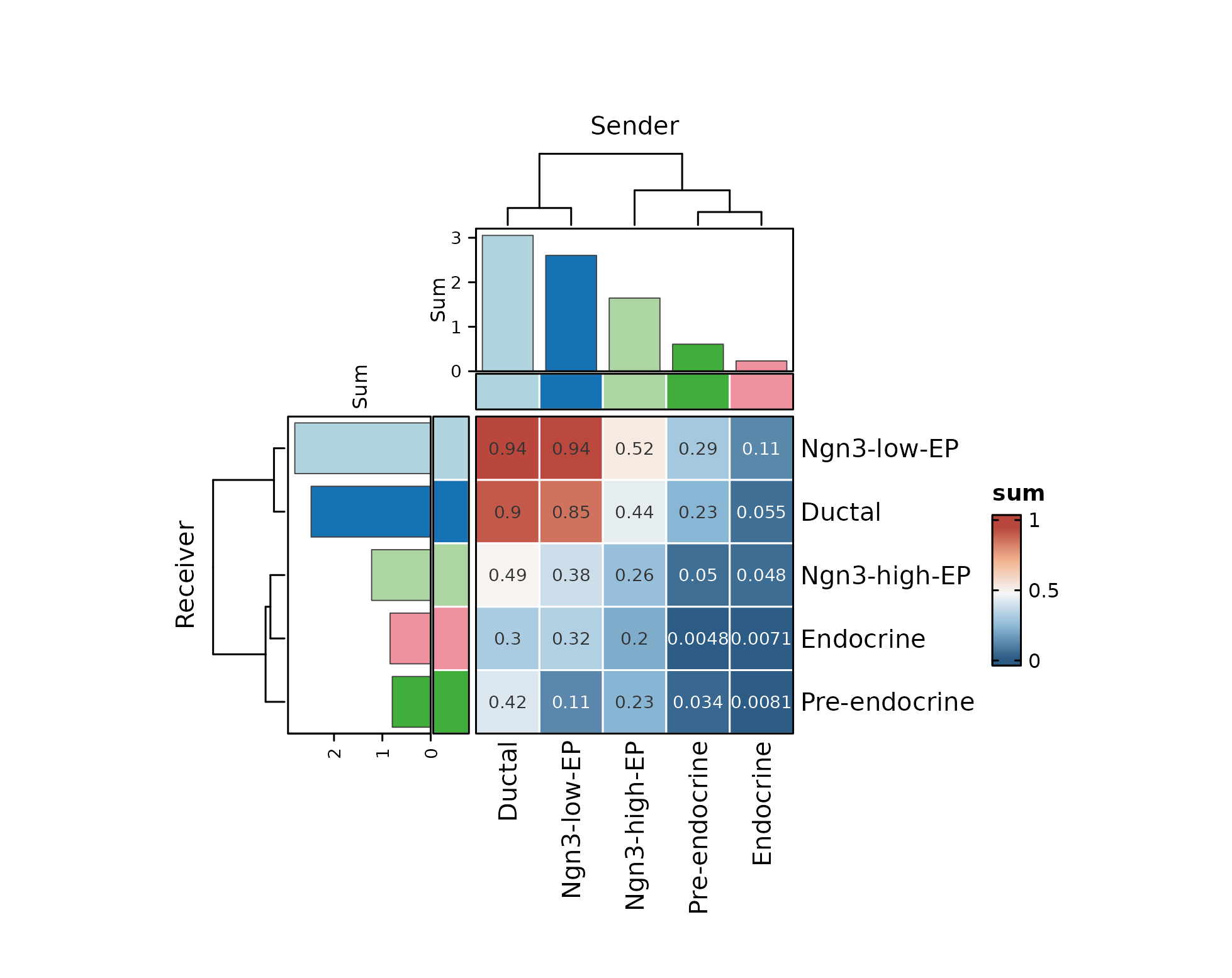
Start with the heatmap layer. A sender-receiver heatmap shows which cell-type pairs have many or strong inferred interactions. In aggregation views, sum summarizes the selected interaction score across retained ligand-receptor events for a sender-receiver pair. Use it to rank cell pairs, then return to the long table to inspect the individual ligands and receptors behind the aggregate signal.

CCCHeatmap(
  pancreas_ccc,
  method = "CCC",
  plot_type = "heatmap",
  display_by = "aggregation",
  value = "sum",
  top_n = 30,
  add_text = TRUE,
  cluster_rows = TRUE,
  cluster_columns = TRUE,
  value_palette = "RdBu",
  value_palcolor = ccc_value_pal,
  cell_palcolor = ccc_cell_pal,
  font.size = 10,
  theme_args = ccc_theme_args
)

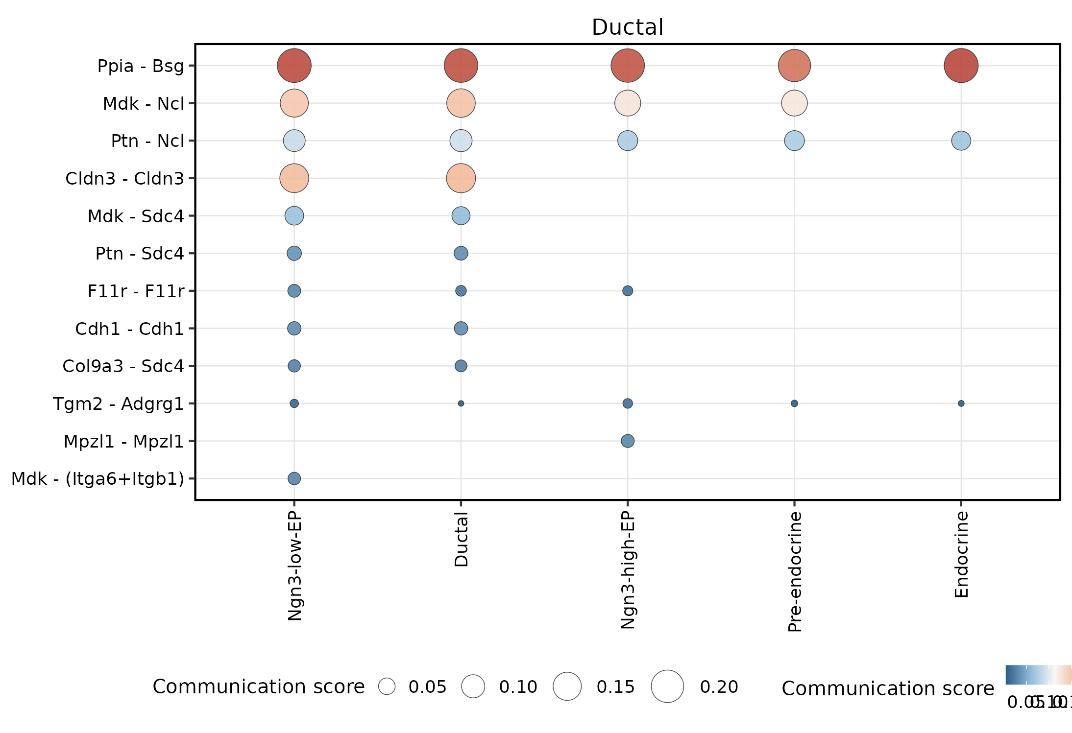
A focused matrix keeps a single sender or receiver readable while preserving interaction names. In static documentation, use small multiples or filters instead of drawing every significant pair at once.

CCCHeatmap(
  pancreas_ccc,
  method = "CCC",
  plot_type = "dot",
  display_by = "interaction",
  sender.use = "Ductal",
  top_n = 12,
  value_palette = "RdBu",
  value_palcolor = ccc_value_pal,
  cell_palcolor = ccc_cell_pal,
  font.size = 9,
  legend.position = "bottom",
  legend.direction = "horizontal",
  theme_args = ccc_theme_args
)

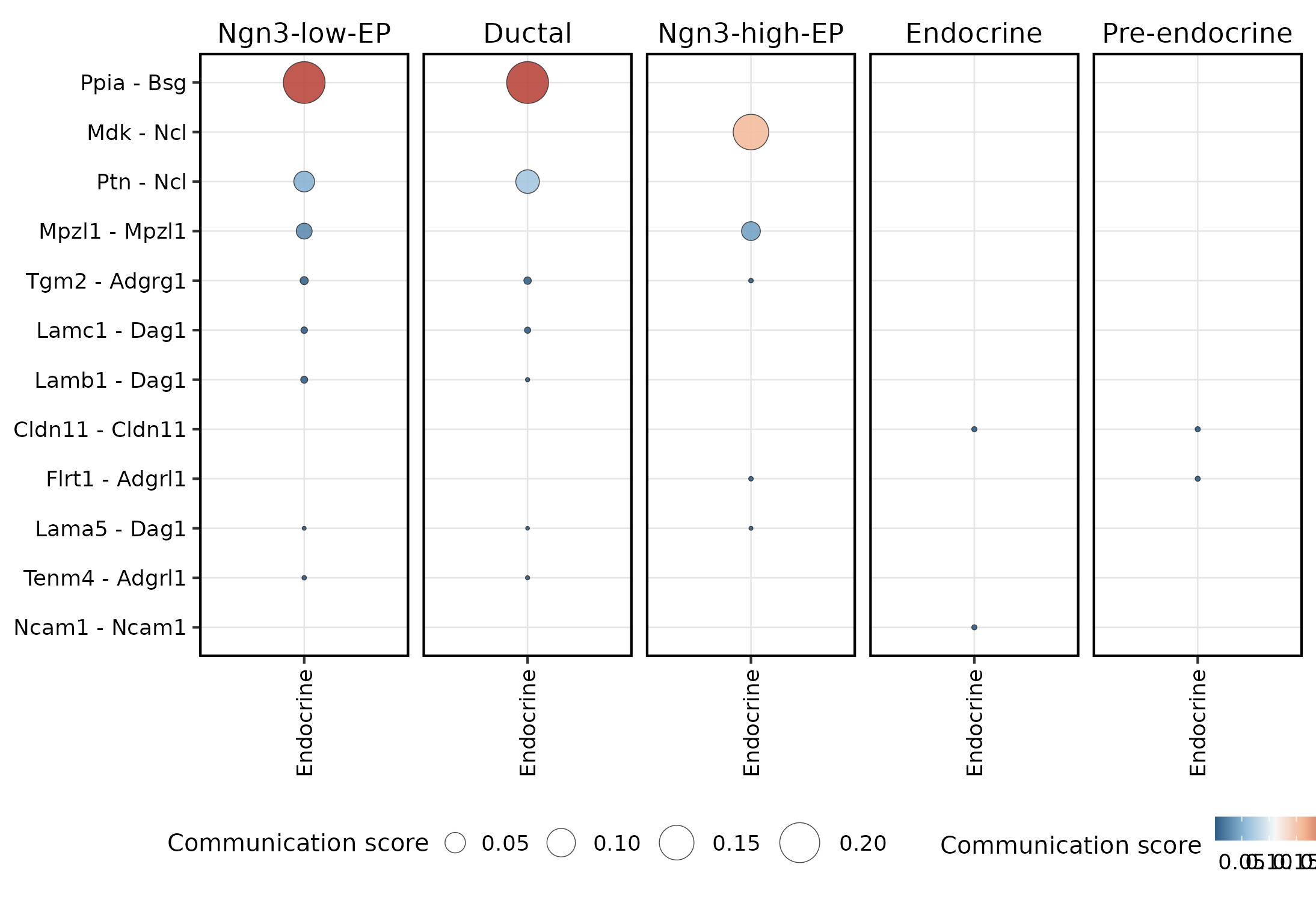
Compare the same interaction-level view from the receiver side. This is useful when a sender-dominant dot plot hides receiver-specific specificity.

CCCHeatmap(
  pancreas_ccc,
  method = "CCC",
  plot_type = "dot",
  display_by = "interaction",
  receiver.use = "Endocrine",
  top_n = 12,
  value_palette = "RdBu",
  value_palcolor = ccc_value_pal,
  cell_palcolor = ccc_cell_pal,
  font.size = 9,
  legend.position = "bottom",
  legend.direction = "horizontal",
  theme_args = ccc_theme_args
)

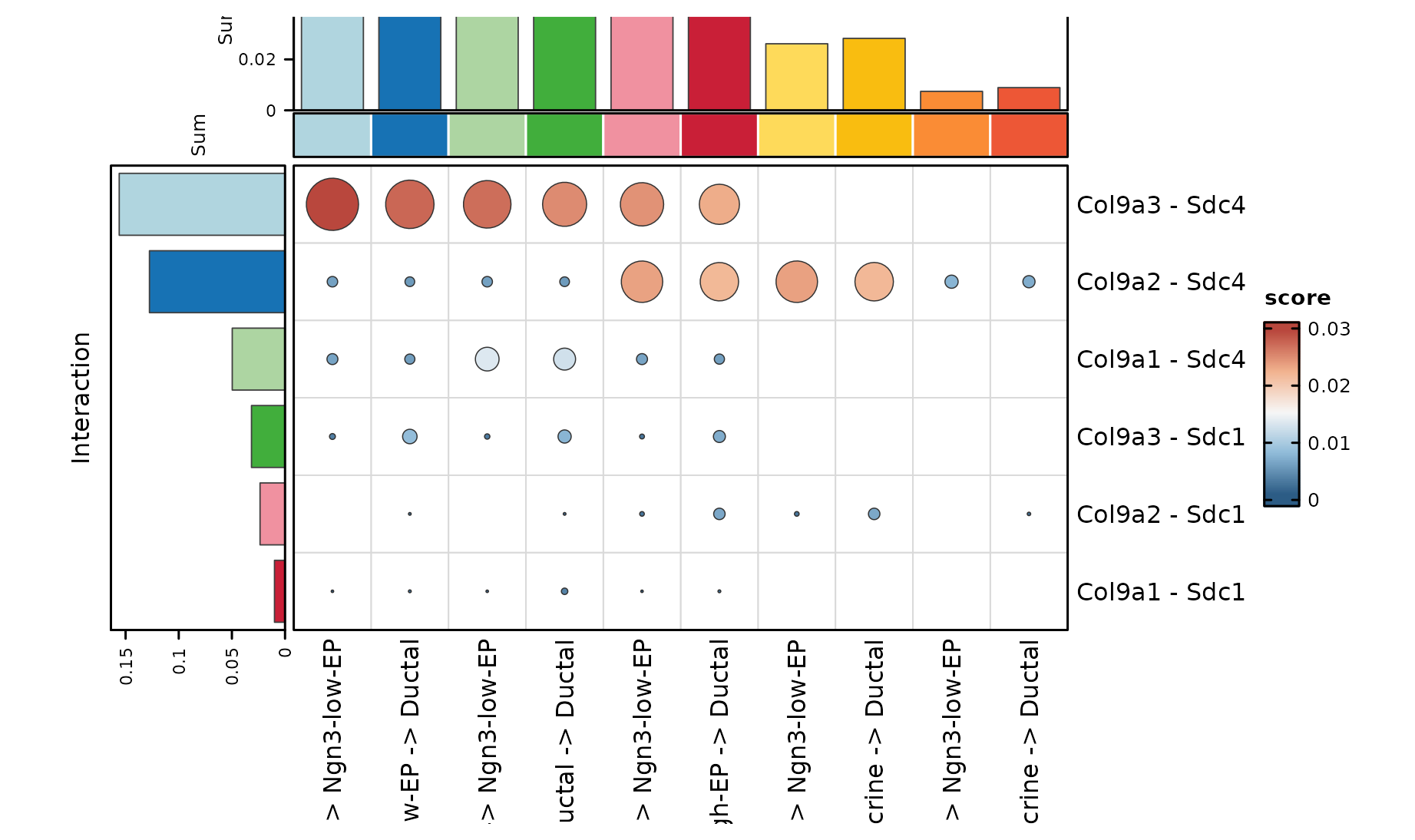
For pathway-level questions, use pathway bubbles before drawing a network. Keep this panel compact in the article because the pathway-specific interaction labels are long. Here a pathway such as COLLAGEN is a ligand-receptor signaling family from the CCC method/resource, not a GO or KEGG enrichment term.

CCCHeatmap(
  pancreas_ccc,
  method = "CCC",
  plot_type = "pathway_bubble",
  display_by = "interaction",
  signaling = "COLLAGEN",
  top_n = 6,
  value_palette = "RdBu",
  value_palcolor = ccc_value_pal,
  cell_palcolor = ccc_cell_pal,
  font.size = 8,
  legend.position = "bottom",
  legend.direction = "horizontal",
  theme_args = ccc_theme_args
)

Statistical Views

Use the statistical layer to decide whether a signal is dominated by a few ligand-receptor pairs or spread across many pairs. pvalue is method-specific and should be interpreted with the method and resource used to generate it. When several CCC methods are combined, use the standardized table for ranking and visualization, but keep method provenance in the report.

CCCStatPlot(
  pancreas_ccc,
  method = "CCC",
  plot_type = "bar",
  display_by = "interaction",
  top_n = 14,
  cell_palcolor = ccc_cell_pal,
  link_palcolor = ccc_cell_pal,
  font.size = 10,
  legend.position = "bottom",
  legend.direction = "horizontal",
  theme_args = ccc_theme_args
)

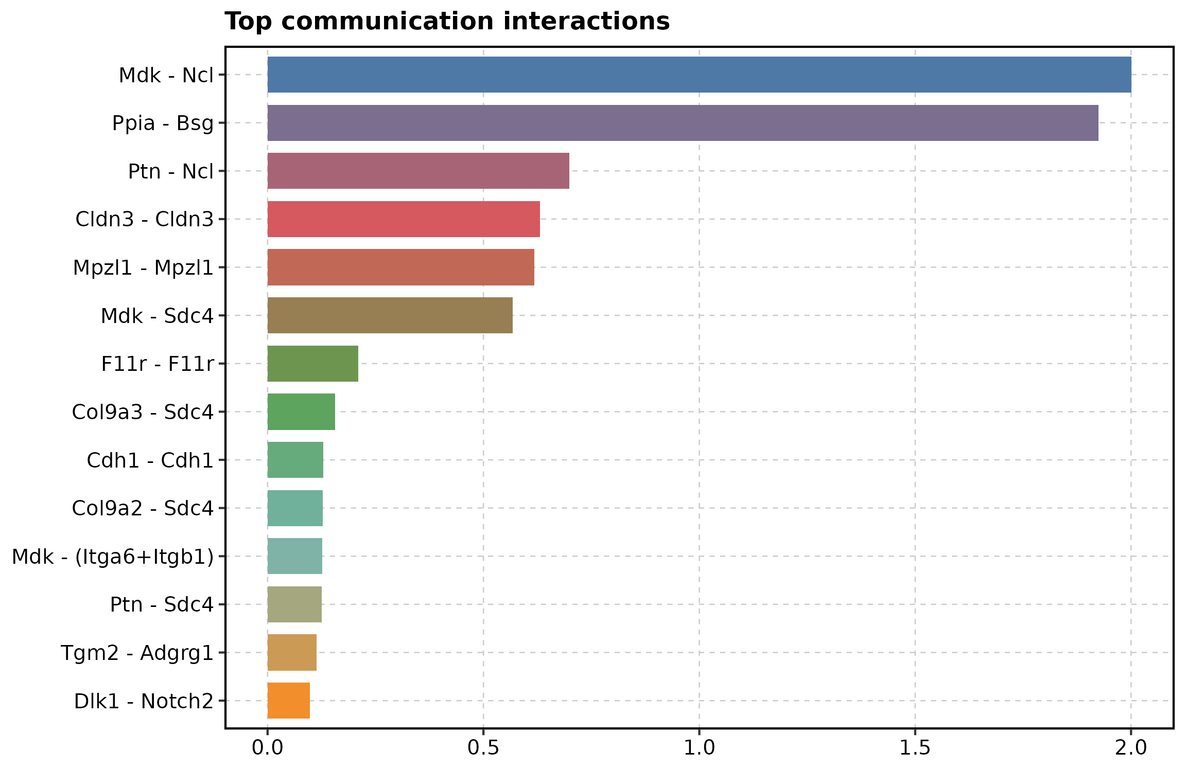
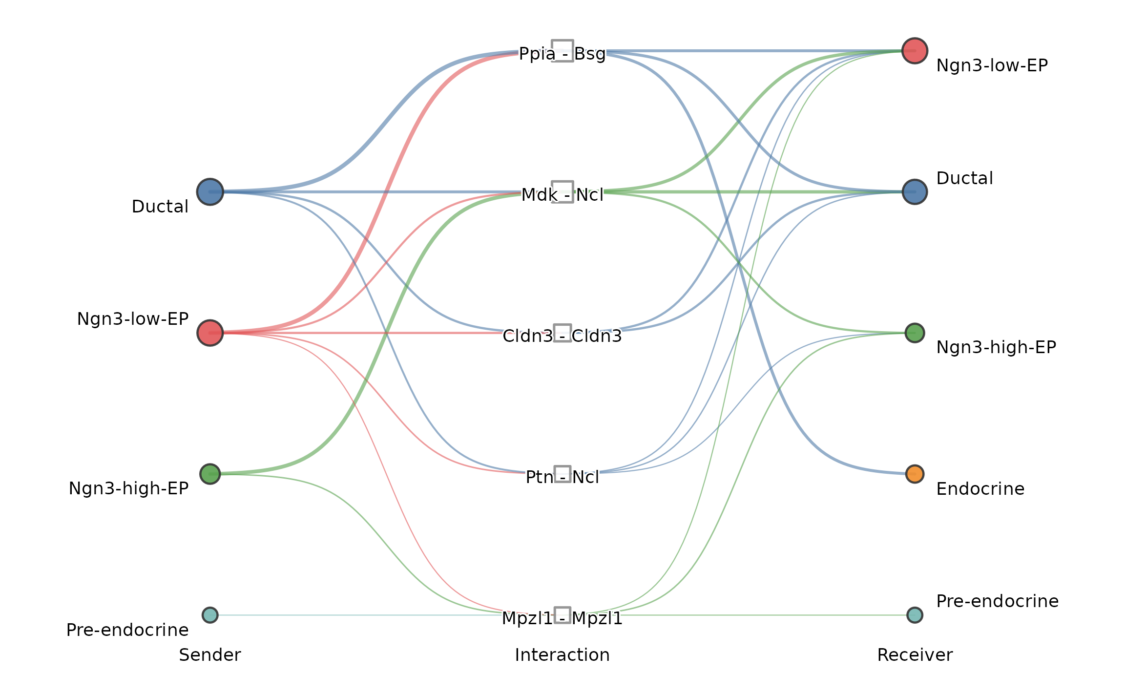
A flow plot is a compact companion to the bar plot: it shows which senders, ligand-receptor interactions, and receivers explain the top-ranked signal. For the article, use a small interaction-level flow with direct labels instead of a dense alluvial panel.

CCCNetworkPlot(
  pancreas_ccc,
  method = "CCC",
  plot_type = "sigmoid",
  display_by = "interaction",
  top_n = 5,
  edge_alpha = 0.5,
  edge_size = c(0.25, 1),
  node_size = 3.8,
  cell_palcolor = ccc_cell_pal,
  link_palcolor = ccc_cell_pal,
  label = TRUE,
  label.size = 3.2,
  label.fg = "black",
  label.bg = "white",
  label.bg.r = 0.12,
  font.size = 9,
  legend.position = "none",
  theme_args = ccc_theme_args
)

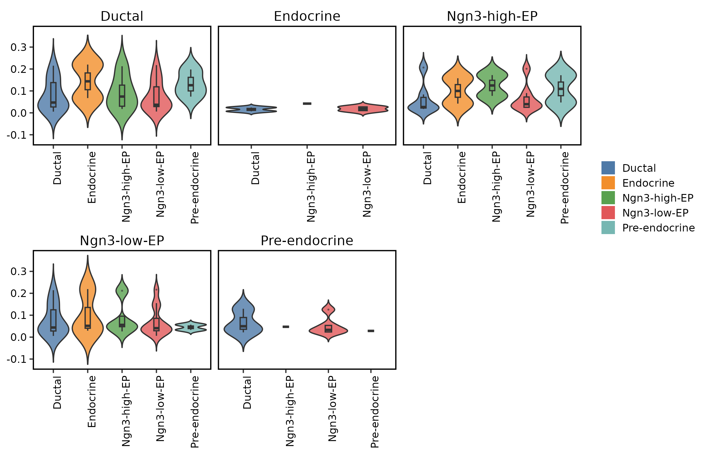
Distribution plots show whether each sender has consistent receiver-side scores or only a few high-scoring outliers. The legend glyphs are simplified so the legend reads as colored categories rather than mini violins.

p_violin <- CCCStatPlot(
  pancreas_ccc,
  method = "CCC",
  plot_type = "violin",
  facet_by = "sender",
  top_n = 12,
  cell_palcolor = ccc_cell_pal,
  font.size = 9,
  legend.position = "right",
  theme_args = ccc_theme_args
)

p_violin +
  ggplot2::guides(
    color = ggplot2::guide_legend(
      override.aes = list(shape = 16, size = 4, linetype = 0, alpha = 1)
    ),
    fill = ggplot2::guide_legend(
      override.aes = list(shape = 22, size = 4, linetype = 0, alpha = 1)
    )
  ) +
  ggplot2::theme(
    legend.key.height = grid::unit(0.35, "cm"),
    legend.key.width = grid::unit(0.35, "cm")
  )

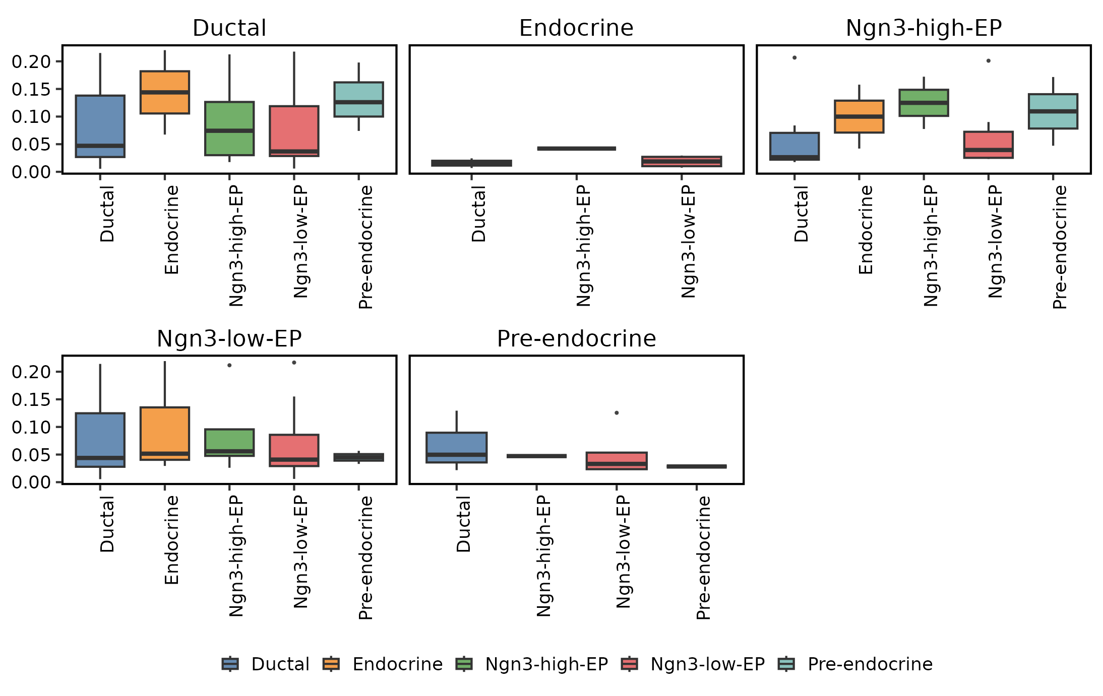
For a global sender-receiver distribution, the box plot is often more compact than faceted violins.

CCCStatPlot(
  pancreas_ccc,
  method = "CCC",
  plot_type = "box",
  top_n = 12,
  cell_palcolor = ccc_cell_pal,
  font.size = 9,
  legend.position = "bottom",
  legend.direction = "horizontal",
  theme_args = ccc_theme_args
)

Network Views

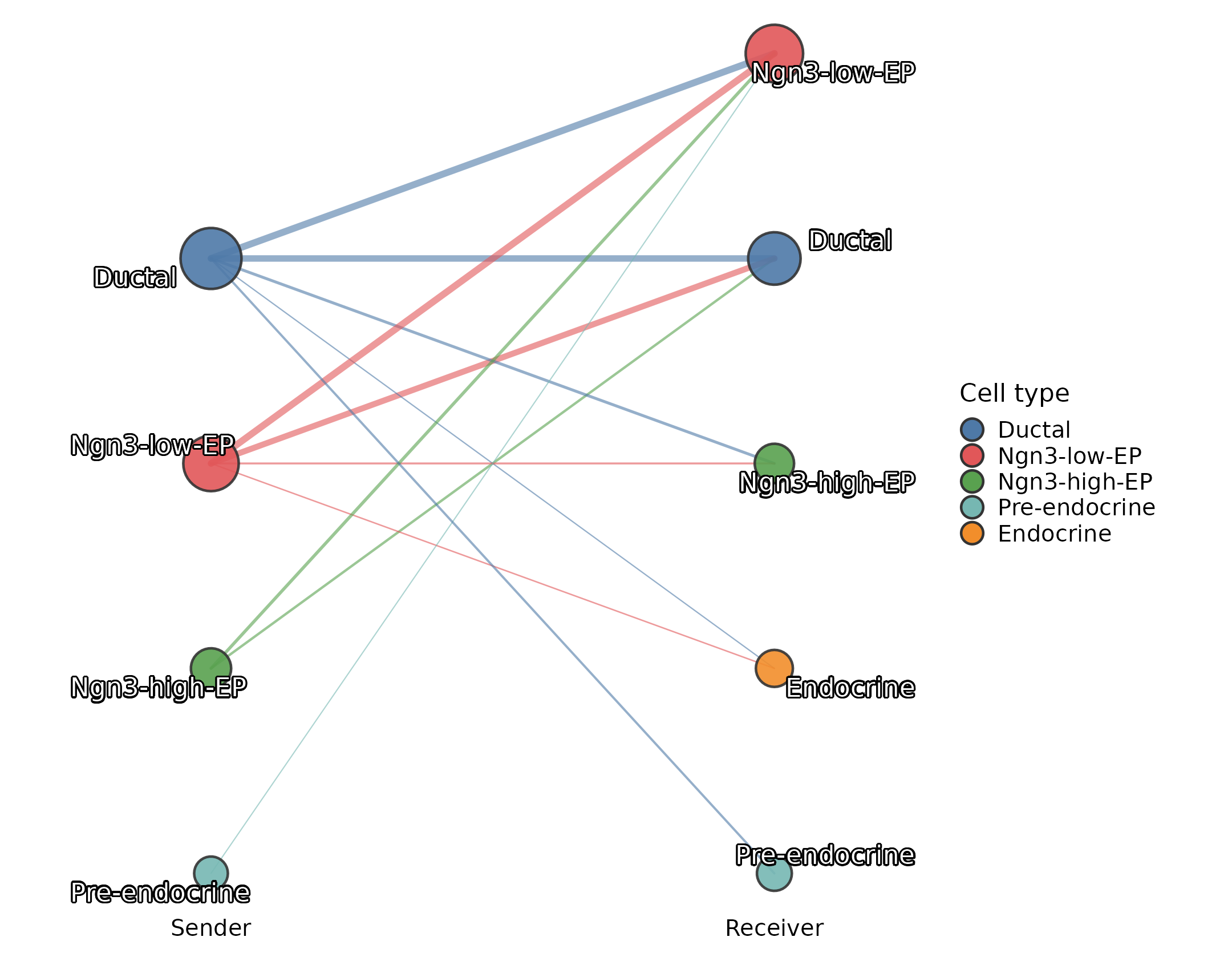
Use the network layer after the global heatmap identifies the cell groups of interest. Aggregate views summarize sender-receiver communication; interaction views show ligand-receptor flow. The compact arrow view is usually easier to read than a dense circle network in an article. Network edge width encodes the selected summary score, and arrows encode sender to receiver direction. The direction is inferred from ligand and receptor group assignment, not from time-course causality.

CCCNetworkPlot(
  pancreas_ccc,
  method = "CCC",
  plot_type = "arrow",
  display_by = "aggregation",
  value = "sum",
  top_n = 12,
  directed = TRUE,
  edge_line = "curved",
  edge_curvature = 0.18,
  edge_alpha = 0.55,
  edge_size = c(0.25, 1.4),
  node_size = 8,
  cell_palcolor = ccc_cell_pal,
  link_palcolor = ccc_cell_pal,
  font.size = 10,
  theme_args = ccc_theme_args
)

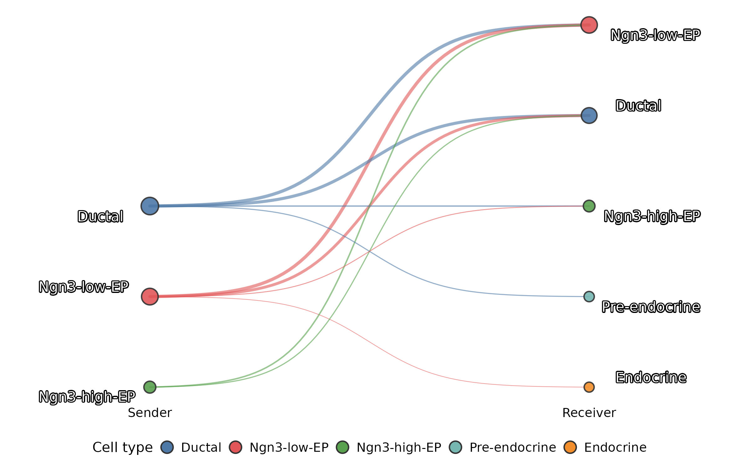
The sigmoid flow view uses the same sender-receiver table but lays it out as columns. It is usually cleaner than a circle when labels are long.

CCCNetworkPlot(
  pancreas_ccc,
  method = "CCC",
  plot_type = "sigmoid",
  display_by = "aggregation",
  value = "sum",
  top_n = 10,
  edge_alpha = 0.55,
  edge_size = c(0.25, 1.2),
  node_size = 4,
  cell_palcolor = ccc_cell_pal,
  link_palcolor = ccc_cell_pal,
  font.size = 10,
  legend.position = "bottom",
  legend.direction = "horizontal",
  theme_args = ccc_theme_args
)

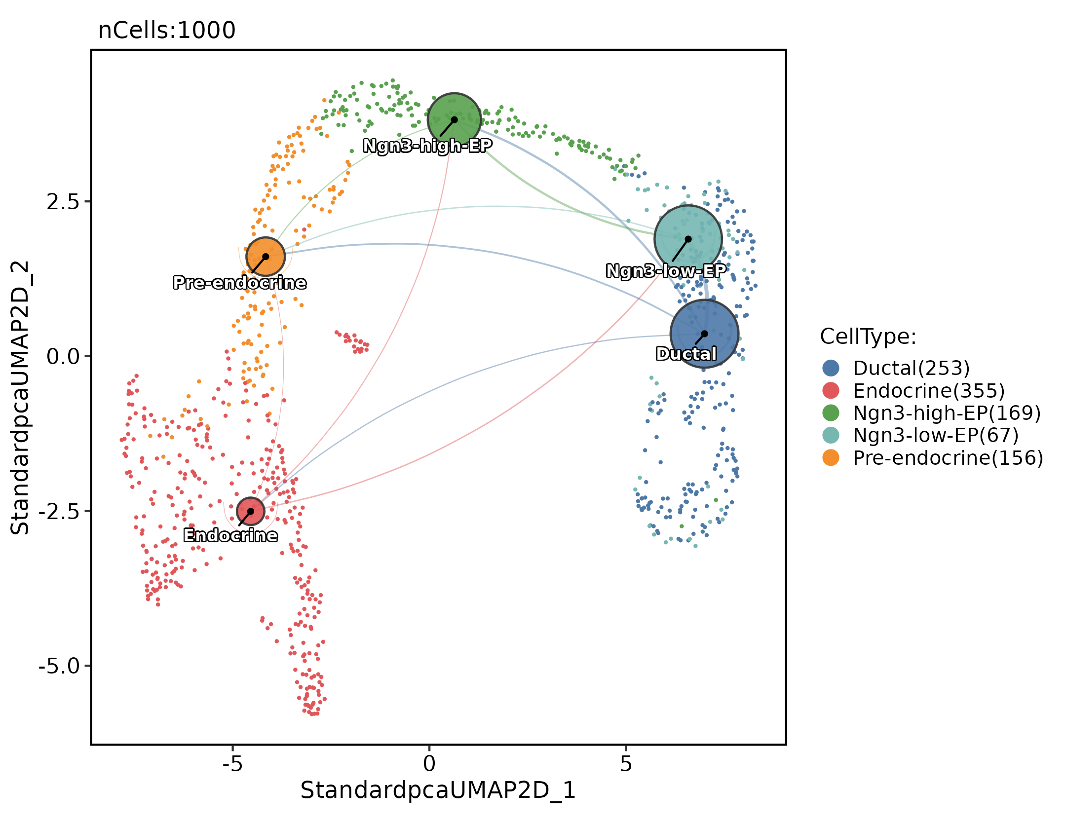
The embedding network overlays sender-receiver links on the cell embedding. This helps distinguish strong communication between nearby cell states from long-range links across transcriptionally distant groups.

CCCNetworkPlot(
  pancreas_ccc,
  method = "CCC",
  plot_type = "embedding_network",
  group.by = "CellType",
  reduction = "Standardumap",
  display_by = "aggregation",
  value = "sum",
  top_n = 12,
  edge_alpha = 0.45,
  edge_size = c(0.15, 0.9),
  node_size = 6,
  cell_palcolor = ccc_cell_pal,
  link_palcolor = ccc_cell_pal,
  font.size = 10,
  label = TRUE,
  label_repel = TRUE,
  label.size = 3,
  theme_args = ccc_theme_args
)

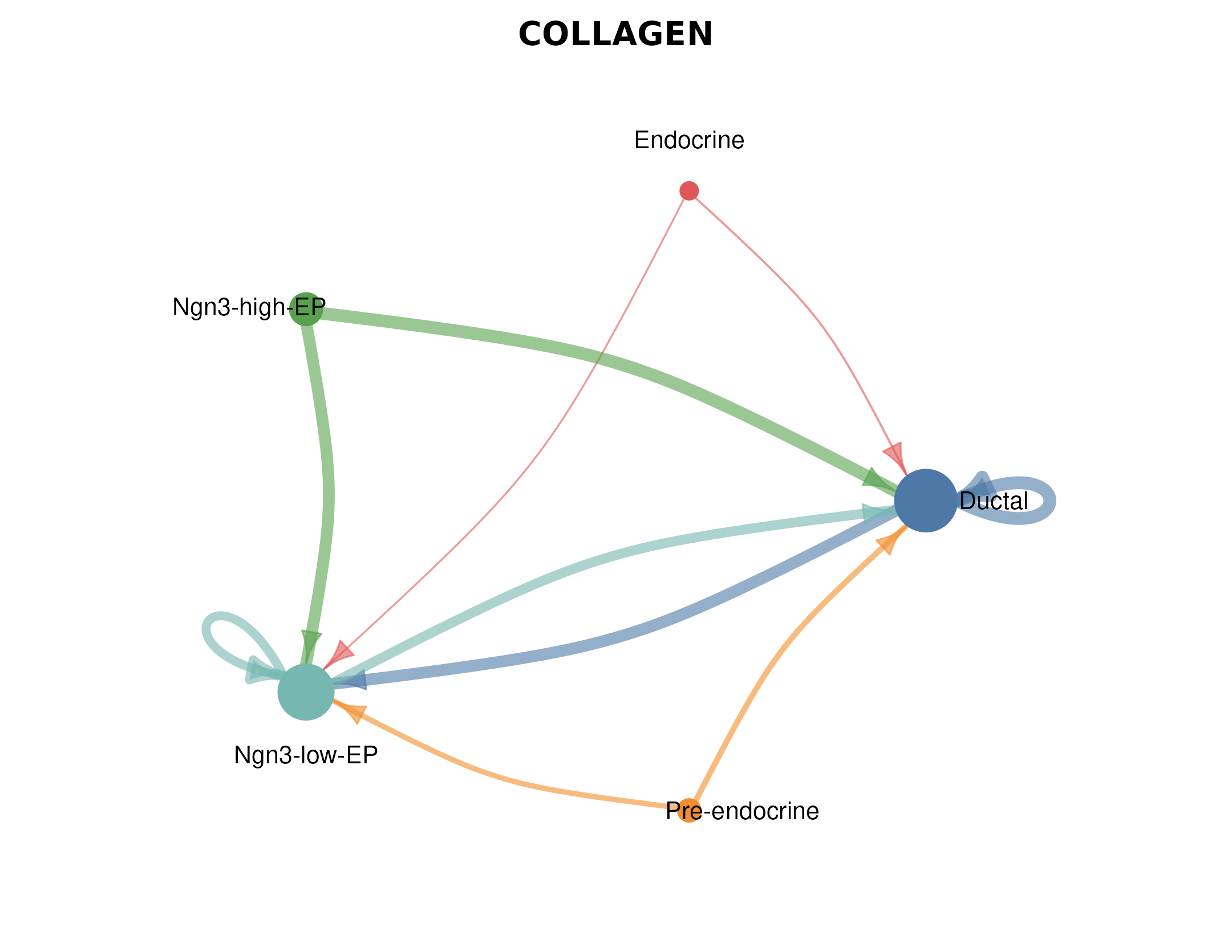
For pathway-aware results, focus on one pathway at a time. This avoids the label overlap that appears when all significant sender-receiver links are drawn in one circle.

CCCNetworkPlot(
  pancreas_ccc,
  method = "CCC",
  plot_type = "pathway",
  signaling = "COLLAGEN",
  display_by = "aggregation",
  value = "sum",
  top_n = 8,
  node_size = 7,
  cell_palcolor = ccc_cell_pal,
  link_palcolor = ccc_cell_pal,
  font.size = 9,
  label.size = 3,
  theme_args = ccc_theme_args
)

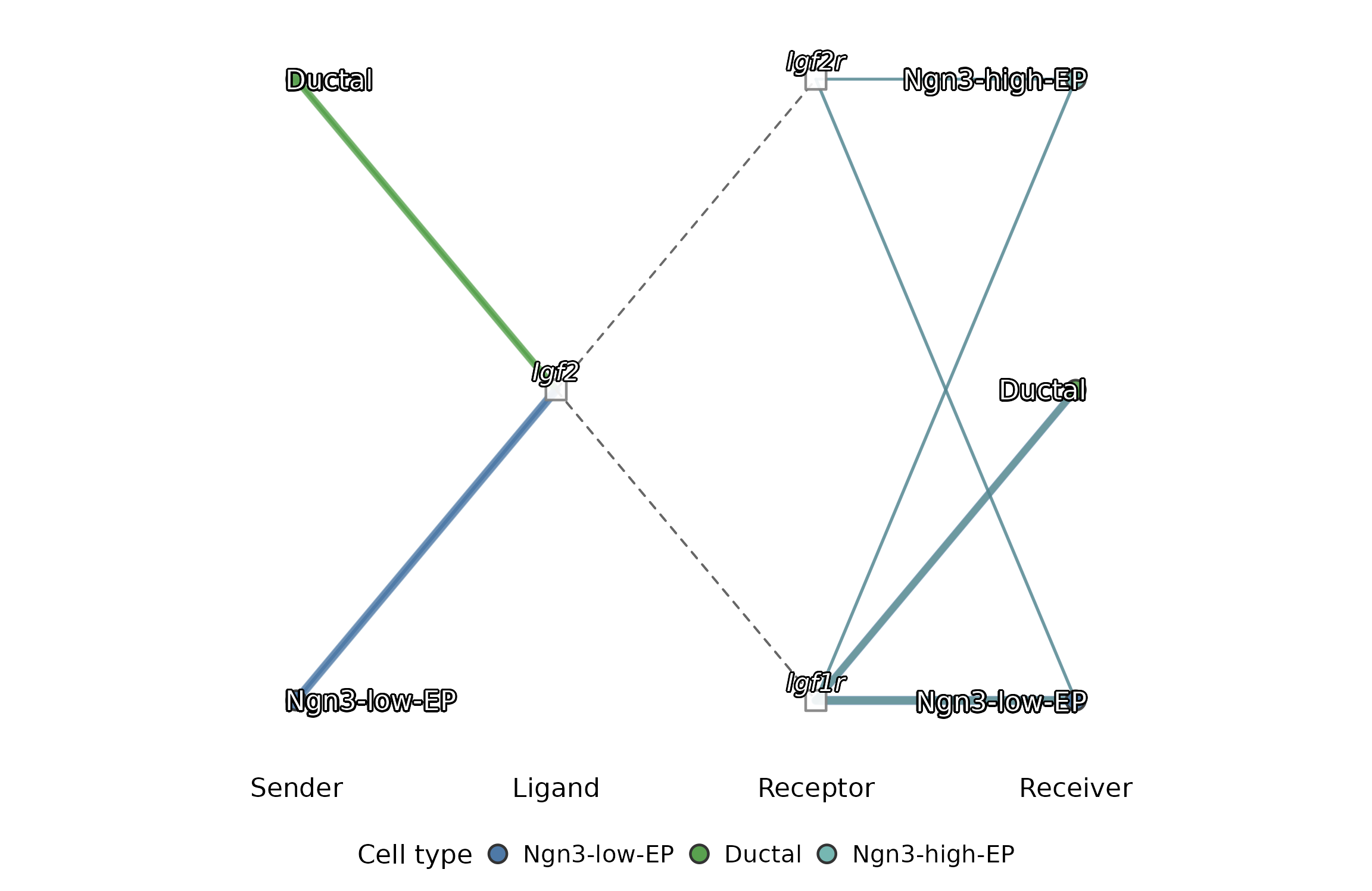
For a focused ligand, the bipartite plot shows the flow from sender groups to the ligand, then to receptors and receiver groups. Keep top_n small when the same ligand has many receiver contexts.

CCCNetworkPlot(
  pancreas_ccc,
  method = "CCC",
  plot_type = "bipartite",
  ligand = "Igf2",
  top_n = 6,
  node_size = 4,
  cell_palcolor = ccc_cell_pal,
  link_palcolor = ccc_cell_pal,
  font.size = 8,
  legend.position = "bottom",
  legend.direction = "horizontal",
  theme_args = ccc_theme_args
)

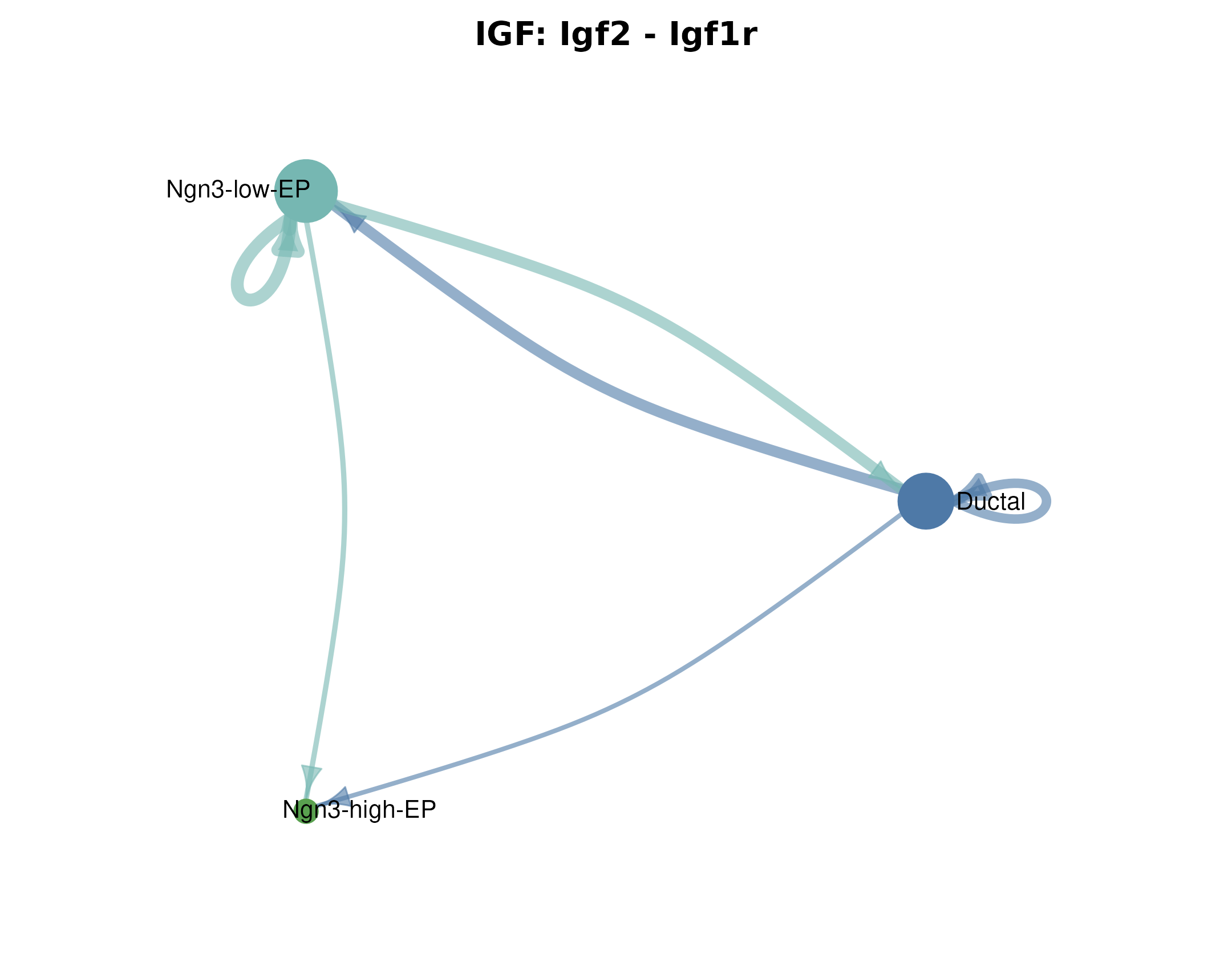
Use a single ligand-receptor pair when the biological question is already specific. The pair name should match interaction_name, pair_lr, or interaction_label in pancreas_ccc@tools$CCC$long_table.

CCCNetworkPlot(
  pancreas_ccc,
  method = "CCC",
  plot_type = "individual_lr",
  signaling = "IGF",
  pairLR.use = "Igf2 - Igf1r",
  display_by = "interaction",
  top_n = 8,
  node_size = 7,
  cell_palcolor = ccc_cell_pal,
  link_palcolor = ccc_cell_pal,
  font.size = 9,
  label.size = 3,
  theme_args = ccc_theme_args
)

The dense circle or chord variants are still useful for interactive inspection, but they are intentionally not drawn here because the full pancreas_sub network is too dense for a static article figure:

CCCNetworkPlot(
  pancreas_ccc,
  method = "CCC",
  plot_type = "circle",
  display_by = "aggregation",
  value = "sum",
  top_n = 8
)

CCCNetworkPlot(
  pancreas_ccc,
  method = "CCC",
  plot_type = "chord",
  display_by = "aggregation",
  top_n = 8
)

Method-Specific R Workflows

Use method-specific wrappers when you need parameters or outputs that are not part of the unified scheduler. CellChat is useful for pathway-level communication and pathway role plots:

pancreas_cellchat <- RunCellChat(
  pancreas_ccc,
  group.by = "CellType",
  species = "Mus_musculus",
  min.cells = 10
)

LIANA is useful when you want several ligand-receptor scoring methods and a consensus-style table:

pancreas_liana <- RunLIANA(
  pancreas_ccc,
  group.by = "CellType",
  method = c("natmi", "connectome", "logfc", "cellphonedb"),
  resource = "Consensus",
  min_cells = 5
)

liana_tbl <- ccc_to_liana(pancreas_liana, method = "LIANA")

For condition comparisons, store the condition in metadata and run CellChat per condition. The comparison output can then be used by differential heatmaps, differential networks, and pathway ranking plots.

pancreas_cmp <- RunCellChat(
  pancreas_ccc,
  group.by = "CellType",
  group_column = "Condition",
  group_cmp = list(c("ConditionA", "ConditionB")),
  species = "Mus_musculus"
)

Link Ligands to Downstream Targets

Use NicheNet when the question is no longer “which cell types communicate?” but “which sender ligands may explain receiver target-gene changes?”. This requires a receiver, sender groups, and either a condition comparison or a custom target gene set.

pancreas_nn <- RunNichenetr(
  pancreas_ccc,
  group.by = "CellType",
  receiver = "Ductal",
  sender = "all",
  condition.by = "Condition",
  condition_oi = "ConditionA",
  condition_reference = "ConditionB",
  mode = "aggregate_cluster_de",
  species = "Mus_musculus"
)

Export R Results

Export a LIANA-style table from the unified CCC result when you want a portable result table for downstream workflows without rebuilding method-specific objects by hand.

liana_res <- ccc_to_liana(
  pancreas_ccc,
  method = "CCC",
  score_col = "score",
  pvalue_col = "pvalue"
)

head(liana_res)
#>   source target    ligand_complex receptor_complex        score pvalue
#> 1 Ductal Ductal              Agrn             Dag1 0.0012782325   0.00
#> 2 Ductal Ductal              Cdh1             Cdh1 0.0323255724   0.00
#> 3 Ductal Ductal              Cdh3             Cdh3 0.0009078211   0.00
#> 4 Ductal Ductal Cholesterol-DHCR7             Rorc 0.0007003888   0.01
#> 5 Ductal Ductal             Cldn3            Cldn3 0.1602736475   0.00
#> 6 Ductal Ductal            Col2a1             Sdc1 0.0012412129   0.00
#>         interaction_name_2       interacting_pair                pair_lr
#> 1              Agrn - Dag1              Agrn_Dag1              Agrn-Dag1
#> 2              Cdh1 - Cdh1              Cdh1_Cdh1              Cdh1-Cdh1
#> 3              Cdh3 - Cdh3              Cdh3_Cdh3              Cdh3-Cdh3
#> 4 Cholesterol-DHCR7 - Rorc Cholesterol-DHCR7_Rorc Cholesterol-DHCR7-Rorc
#> 5            Cldn3 - Cldn3            Cldn3_Cldn3            Cldn3-Cldn3
#> 6            Col2a1 - Sdc1            Col2a1_Sdc1            Col2a1-Sdc1
#>                     interaction_name classification   method dataset
#> 1                          AGRN_DAG1           AGRN CellChat     ALL
#> 2                          CDH1_CDH1            CDH CellChat     ALL
#> 3                          CDH3_CDH3            CDH CellChat     ALL
#> 4 Cholesterol-Cholesterol-DHCR7_RORC    Cholesterol CellChat     ALL
#> 5                        CLDN3_CLDN3           CLDN CellChat     ALL
#> 6                        COL2A1_SDC1       COLLAGEN CellChat     ALL
#>   specificity_rank magnitude_rank aggregate_rank
#> 1              245            245           0.00
#> 2               59             59           0.00
#> 3              266            266           0.00
#> 4              268            268           0.01
#> 5               14             14           0.00
#> 6              248            248           0.00

What to Report

A compact CCC report should include:

the object, assay, expression layer, and sender-receiver annotation;
the method or methods used, including species and ligand-receptor resource;
the significance threshold and expression fraction cutoff;
the top sender-receiver pairs by interaction count or score;
the top ligand-receptor pairs, separated from aggregate cell-pair summaries;
whether the result is steady-state communication or a condition comparison;
downstream target interpretation only when using a method designed for that question, such as NicheNet.

Keep the first pass broad and conservative. Use focused ligand, receptor, pathway, and downstream target analyses only after the global sender-receiver structure is stable.