Visualize cell groups on a 2-dimensional reduction plot. Plotting cell points on a reduced 2D plane and coloring according to the groups.
Usage
CellDimPlot(
  srt,
  group.by,
  label.by = NULL,
  mark.by = NULL,
  legend.by = NULL,
  reduction = NULL,
  dims = c(1, 2),
  split.by = NULL,
  cells = NULL,
  show_na = FALSE,
  show_stat = ifelse(identical(theme_use, "theme_blank"), FALSE, TRUE),
  pt.size = NULL,
  pt.alpha = 1,
  palette = "Chinese",
  palcolor = NULL,
  bg_color = "grey80",
  label = FALSE,
  label.size = 4,
  label.fg = "white",
  label.bg = "black",
  label.bg.r = 0.1,
  label_insitu = FALSE,
  label_repel = FALSE,
  label_repulsion = 20,
  label_point_size = 1,
  label_point_color = "black",
  label_segment_color = "black",
  cells.highlight = NULL,
  cols.highlight = "black",
  sizes.highlight = 1,
  alpha.highlight = 1,
  stroke.highlight = 0.5,
  add_density = FALSE,
  density_color = "grey80",
  density_filled = FALSE,
  density_filled_palette = "Greys",
  density_filled_palcolor = NULL,
  add_mark = FALSE,
  mark_type = c("hull", "ellipse", "rect", "circle"),
  mark_expand = grid::unit(3, "mm"),
  mark_alpha = 0.1,
  mark_linetype = 1,
  mark_linewidth = 0.5,
  mark_border = NULL,
  mark_palette = palette,
  mark_palcolor = NULL,
  add_grid = FALSE,
  grid_n = 12,
  grid_color = "black",
  grid_size = 0.25,
  grid_alpha = 0.35,
  lineages = NULL,
  lineages_trim = c(0.01, 0.99),
  lineages_span = 0.75,
  lineages_palette = "Dark2",
  lineages_palcolor = NULL,
  lineages_arrow = grid::arrow(length = grid::unit(0.1, "inches")),
  lineages_linewidth = 1,
  lineages_line_bg = "white",
  lineages_line_bg_stroke = 0.5,
  lineages_whiskers = FALSE,
  lineages_whiskers_linewidth = 0.5,
  lineages_whiskers_alpha = 0.5,
  stat.by = NULL,
  stat_type = "percent",
  stat_plot_type = "pie",
  stat_plot_position = c("stack", "dodge"),
  stat_plot_size = 0.2,
  stat_plot_palette = "Set1",
  stat_palcolor = NULL,
  stat_plot_alpha = 1,
  stat_plot_label = FALSE,
  stat_plot_label_size = 3,
  graph = NULL,
  edge_size = c(0.05, 0.5),
  edge_alpha = 0.1,
  edge_color = "grey40",
  paga = NULL,
  paga_type = "connectivities",
  paga_node_size = 4,
  paga_edge_threshold = 0.01,
  paga_edge_size = c(0.2, 1),
  paga_edge_color = "grey40",
  paga_edge_alpha = 0.5,
  paga_transition_threshold = 0.01,
  paga_transition_size = c(0.2, 1),
  paga_transition_color = "black",
  paga_transition_alpha = 1,
  paga_show_transition = FALSE,
  velocity = NULL,
  velocity_plot_type = "raw",
  velocity_n_neighbors = ceiling(ncol(srt@assays[[1]])/50),
  velocity_density = 1,
  velocity_smooth = 0.5,
  velocity_scale = 1,
  velocity_min_mass = 1,
  velocity_cutoff_perc = 5,
  velocity_arrow_color = "black",
  velocity_arrow_angle = 20,
  streamline_L = 5,
  streamline_minL = 1,
  streamline_res = 1,
  streamline_n = 15,
  streamline_width = c(0, 0.8),
  streamline_alpha = 1,
  streamline_color = NULL,
  streamline_palette = "RdYlBu",
  streamline_palcolor = NULL,
  streamline_bg_color = "white",
  streamline_bg_stroke = 0.5,
  hex = FALSE,
  hex.linewidth = 0.5,
  hex.count = TRUE,
  hex.bins = 50,
  hex.binwidth = NULL,
  raster = NULL,
  raster.dpi = c(512, 512),
  aspect.ratio = 1,
  title = NULL,
  subtitle = NULL,
  xlab = NULL,
  ylab = NULL,
  legend.position = "right",
  legend.direction = "vertical",
  legend.title = NULL,
  theme_use = "theme_scop",
  theme_args = list(),
  combine = TRUE,
  nrow = NULL,
  ncol = NULL,
  byrow = TRUE,
  force = FALSE,
  seed = 11,
  verbose = TRUE
)
Arguments
- srt
A Seurat object.
- group.by
Name of one or more meta.data columns to group (color) cells by.
- label.by
Name of a meta.data column used to place group labels. If
NULL, labels usegroup.by.- mark.by
Name of a meta.data column used to draw group marks. If
NULL, marks uselegend.bywhen a nested legend is requested, otherwise marks usegroup.by.- legend.by
Name of a meta.data column used as the parent group in a nested legend. The
group.bylevels are shown under eachlegend.bylevel. IfNULL, the standard legend is used.- reduction
Which dimensionality reduction to use. If not specified, will use the reduction returned by DefaultReduction.
- dims
Dimensions to plot, must be a two-length numeric vector specifying x- and y-dimensions
- split.by
Name of a column in meta.data column to split plot by. Default is
NULL.- cells
A character vector of cell names to use.
- show_na
Whether to assign a color from the color palette to NA group. If
TRUE, cell points with NA level will be colored bybg_color. IfFALSE, cell points with NA level will be removed from the plot.- show_stat
Whether to show statistical information on the plot.
- pt.size
The size of the points in the plot. Default is
NULL, which automatically scales point diameter with the square root of the number of plotted cells.- pt.alpha
The transparency of the data points. Default is
1.- palette
Color palette name. Available palettes can be found in thisplot::show_palettes. Default is
"Chinese".- palcolor
Custom colors used to create a color palette. Default is
NULL.- bg_color
Color value for background(NA) points.
- label
Whether to label the cell groups.
- label.size
Size of labels.
- label.fg
Foreground color of label.
- label.bg
Background color of label.
- label.bg.r
Background ratio of label.
- label_insitu
Whether to place the raw labels (group names) in the center of the cells with the corresponding group. Default is
FALSE, which using numbers instead of raw labels.- label_repel
Logical value indicating whether the label is repel away from the center points.
- label_repulsion
Force of repulsion between overlapping text labels. Default is
20.- label_point_size
Size of the center points.
- label_point_color
Color of the center points.
- label_segment_color
Color of the line segment for labels.
- cells.highlight
A logical or character vector specifying the cells to highlight in the plot. If
TRUE, all cells are highlighted. IfFALSE, no cells are highlighted. Default isNULL.- cols.highlight
Color used to highlight the cells.
- sizes.highlight
Size of highlighted cell points.
- alpha.highlight
Transparency of highlighted cell points.
- stroke.highlight
Border width of highlighted cell points.
- add_density
Whether to add a density layer on the plot.
- density_color
Color of the density contours lines.
- density_filled
Whether to add filled contour bands instead of contour lines.
- density_filled_palette
Color palette used to fill contour bands.
- density_filled_palcolor
Custom colors used to fill contour bands.
- add_mark
Whether to add marks around cell groups. Default is
FALSE.- mark_type
Type of mark to add around cell groups. One of "hull", "ellipse", "rect", or "circle". Default is
"hull".- mark_expand
Expansion of the mark around the cell group. Default is
grid::unit(3, "mm").- mark_alpha
Transparency of the mark. Default is
0.1.- mark_linetype
Line type of the mark border. Default is
1(solid line).- mark_linewidth
Line width of the mark border.
- mark_border
Fixed border color for marks. If
NULL, mark borders use the group colors.- mark_palette
Color palette name for
mark.bygroups and nested legend parent headers. Defaults topalette.- mark_palcolor
Custom colors for
mark.bygroups and nested legend parent headers.- add_grid
Whether to add a background point grid on the reduction panel. This is useful for atlas-style panels with blank axes.
- grid_n
Number of grid points along each axis when
add_grid = TRUE.- grid_color, grid_size, grid_alpha
Color, size, and alpha of the background grid points.
- lineages
Lineages/pseudotime to add to the plot. If specified, curves will be fitted using stats::loess method.
- lineages_trim
Trim the leading and the trailing data in the lineages.
- lineages_span
The parameter α which controls the degree of smoothing in stats::loess method.
- lineages_palette
Color palette used for lineages.
- lineages_palcolor
Custom colors used for lineages.
- lineages_arrow
Set arrows of the lineages. See grid::arrow.
- lineages_linewidth
Width of fitted curve lines for lineages.
- lineages_line_bg
Background color of curve lines for lineages.
- lineages_line_bg_stroke
Border width of curve lines background.
- lineages_whiskers
Whether to add whiskers for lineages.
- lineages_whiskers_linewidth
Width of whiskers for lineages.
- lineages_whiskers_alpha
Transparency of whiskers for lineages.
- stat.by
The name of a metadata column to stat.
- stat_type
Set stat types ("percent" or "count").
- stat_plot_type
Set the statistical plot type.
- stat_plot_position
Position adjustment in statistical plot.
- stat_plot_size
Set the statistical plot size. Default is
0.2.- stat_plot_palette
Color palette used in statistical plot.
- stat_palcolor
Custom colors used in statistical plot
- stat_plot_alpha
Transparency of the statistical plot.
- stat_plot_label
Whether to add labels in the statistical plot.
- stat_plot_label_size
Label size in the statistical plot.
- graph
Specify the graph name to add edges between cell neighbors to the plot.
- edge_size
Size of edges.
- edge_alpha
Transparency of edges.
- edge_color
Color of edges.
- paga
Specify the calculated paga results to add a PAGA graph layer to the plot.
- paga_type
PAGA plot type. "connectivities" or "connectivities_tree".
- paga_node_size
Size of the nodes in PAGA plot.
- paga_edge_threshold
Threshold of edge connectivities in PAGA plot.
- paga_edge_size
Size of edges in PAGA plot.
- paga_edge_color
Color of edges in PAGA plot.
- paga_edge_alpha
Transparency of edges in PAGA plot.
- paga_transition_threshold
Threshold of transition edges in PAGA plot.
- paga_transition_size
Size of transition edges in PAGA plot.
- paga_transition_color
Color of transition edges in PAGA plot.
- paga_transition_alpha
Transparency of transition edges in PAGA plot.
- paga_show_transition
Whether to show transitions between edges.
- velocity
Specify the calculated RNA velocity mode to add a velocity layer to the plot.
- velocity_plot_type
Set the velocity plot type.
- velocity_n_neighbors
Set the number of neighbors used in velocity plot.
- velocity_density
Set the density value used in velocity plot.
- velocity_smooth
Set the smooth value used in velocity plot.
- velocity_scale
Set the scale value used in velocity plot.
- velocity_min_mass
Set the min_mass value used in velocity plot.
- velocity_cutoff_perc
Set the cutoff_perc value used in velocity plot.
- velocity_arrow_color
Color of arrows in velocity plot.
- velocity_arrow_angle
Angle of arrows in velocity plot.
- streamline_L
Typical length of a streamline in x and y units
- streamline_minL
Minimum length of segments to show.
- streamline_res
Resolution parameter (higher numbers increases the resolution).
- streamline_n
Number of points to draw.
- streamline_width
Size of streamline.
- streamline_alpha
Transparency of streamline.
- streamline_color
Color of streamline.
- streamline_palette
Color palette used for streamline.
- streamline_palcolor
Custom colors used for streamline.
- streamline_bg_color
Background color of streamline.
- streamline_bg_stroke
Border width of streamline background.
- hex
Whether to chane the plot type from point to the hexagonal bin.
- hex.linewidth
Border width of hexagonal bins.
- hex.count
Whether show cell counts in each hexagonal bin.
- hex.bins
Number of hexagonal bins.
- hex.binwidth
Hexagonal bin width.
- raster
Convert points to raster format. Default is
NULL, which automatically rasterizes if plotting more than 100,000 cells.- raster.dpi
Pixel resolution for rasterized plots. Default is
c(512, 512).- aspect.ratio
Aspect ratio of the panel. Default is
1.- title
The text for the title. Default is
NULL.- subtitle
The text for the subtitle for the plot which will be displayed below the title. Default is
NULL.- xlab
The x-axis label of the plot. Default is
NULL.- ylab
The y-axis label of the plot. Default is
NULL.- legend.position
The position of legends, one of
"none","left","right","bottom","top". Default is"right".- legend.direction
The direction of the legend in the plot. Can be one of
"vertical"or"horizontal".- legend.title
Title for the legend. Default is
NULL, which uses the group name.- theme_use
Theme used. Can be a character string or a theme function. Default is
"theme_scop".- theme_args
Other arguments passed to the
theme_use. Default islist().- combine
Combine plots into a single
patchworkobject. IfFALSE, return a list of ggplot objects.- nrow
Number of rows in the combined plot. Default is
NULL, which means determined automatically based on the number of plots.- ncol
Number of columns in the combined plot. Default is
NULL, which means determined automatically based on the number of plots.- byrow
Whether to arrange the plots by row in the combined plot. Default is
TRUE.- force
Whether to force drawing regardless of maximum levels in any cell group is greater than 100. Default is
FALSE.- seed
Random seed for reproducibility. Default is
11.- verbose
Whether to print the message. Default is
TRUE.
Examples
data(pancreas_sub)
pancreas_sub <- standard_scop(pancreas_sub)
#> ℹ [2026-07-22 10:29:12] Start standard processing workflow...
#> ℹ [2026-07-22 10:29:12] Checking a list of <Seurat>...
#> ! [2026-07-22 10:29:12] Data 1/1 of the `srt_list` is "unknown"
#> ℹ [2026-07-22 10:29:12] Perform `NormalizeData()` with `normalization.method = 'LogNormalize'` on 1/1 of `srt_list`...
#> ℹ [2026-07-22 10:29:12] Perform `FindVariableFeatures()` on 1/1 of `srt_list`...
#> ℹ [2026-07-22 10:29:12] Use the separate HVF from `srt_list`
#> ℹ [2026-07-22 10:29:12] Number of available HVF: 2000
#> ℹ [2026-07-22 10:29:12] Finished check
#> ℹ [2026-07-22 10:29:12] Perform `ScaleData()`
#> ℹ [2026-07-22 10:29:13] Perform pca linear dimension reduction
#> ℹ [2026-07-22 10:29:14] Use stored estimated dimensions 1:23 for Standardpca
#> ℹ [2026-07-22 10:29:15] Perform `Seurat::FindClusters()` with `cluster_algorithm = 'louvain'` and `cluster_resolution = 0.6`
#> ℹ [2026-07-22 10:29:15] Reorder clusters...
#> ℹ [2026-07-22 10:29:15] Skip `log1p()` because `layer = data` is not "counts"
#> ℹ [2026-07-22 10:29:15] Perform umap nonlinear dimension reduction
#> ✔ [2026-07-22 10:29:20] Standard processing workflow completed
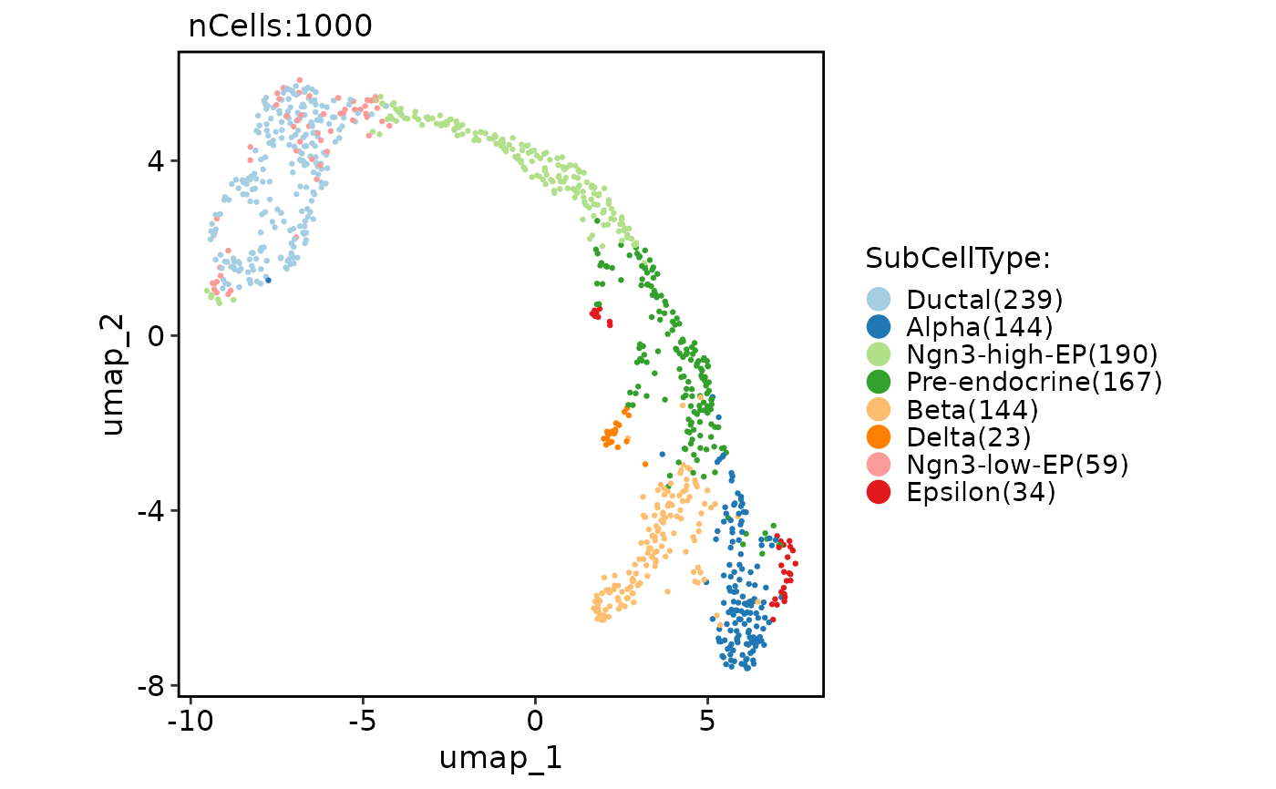
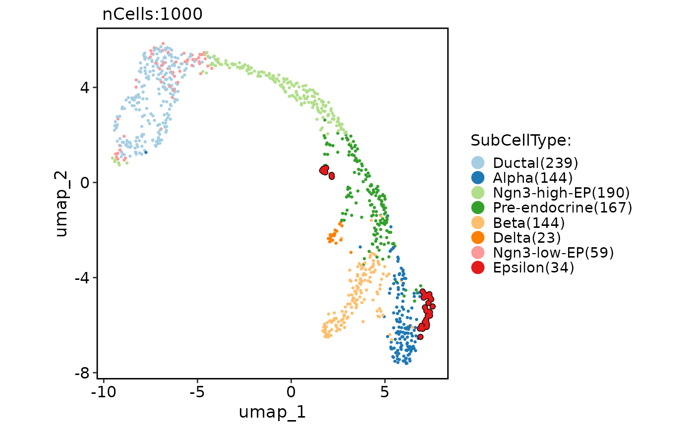
p1 <- CellDimPlot(
pancreas_sub,
group.by = "SubCellType",
reduction = "UMAP"
)
p1
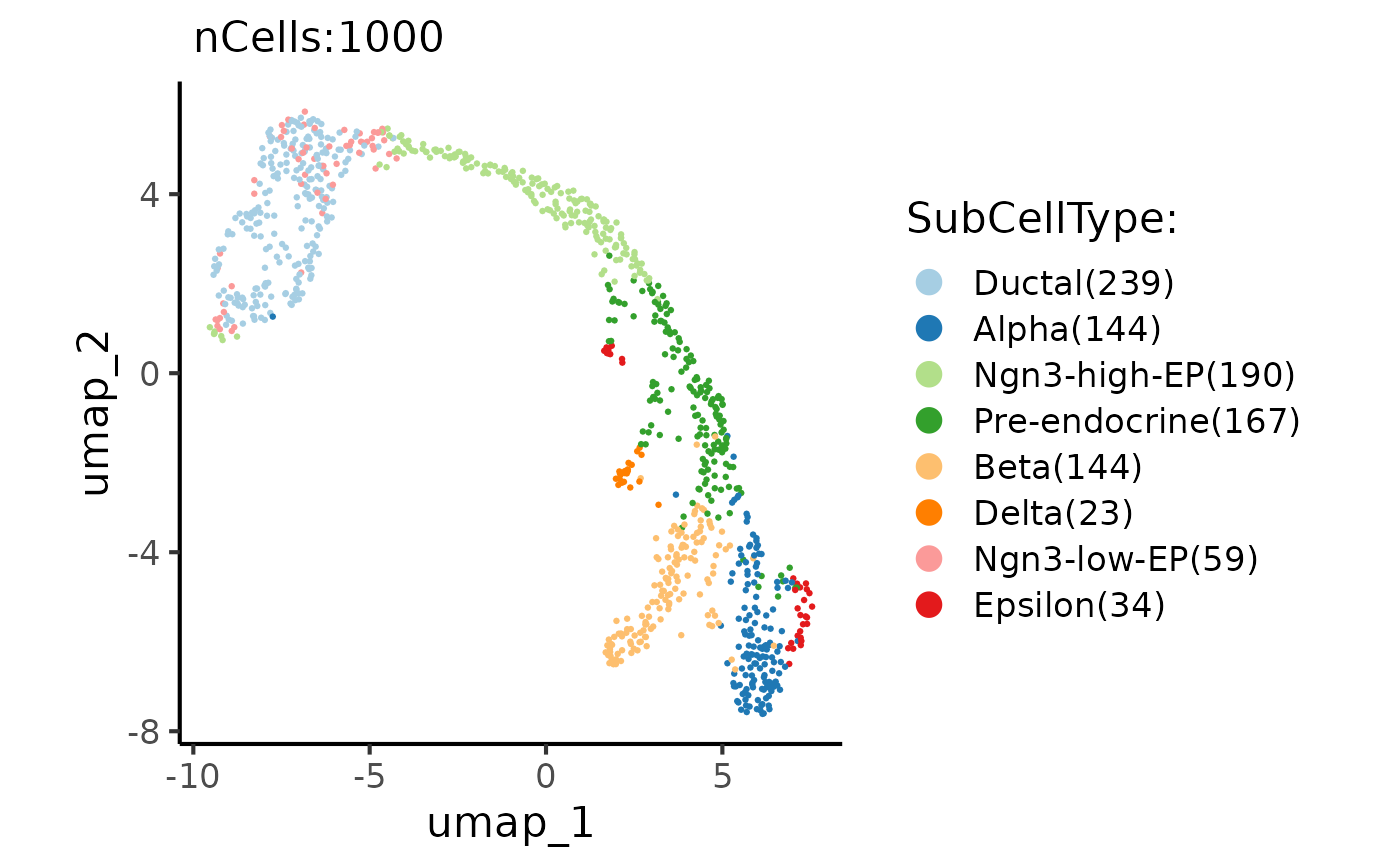
 thisplot::panel_fix(
p1,
height = 2,
raster = TRUE,
dpi = 300
)
thisplot::panel_fix(
p1,
height = 2,
raster = TRUE,
dpi = 300
)
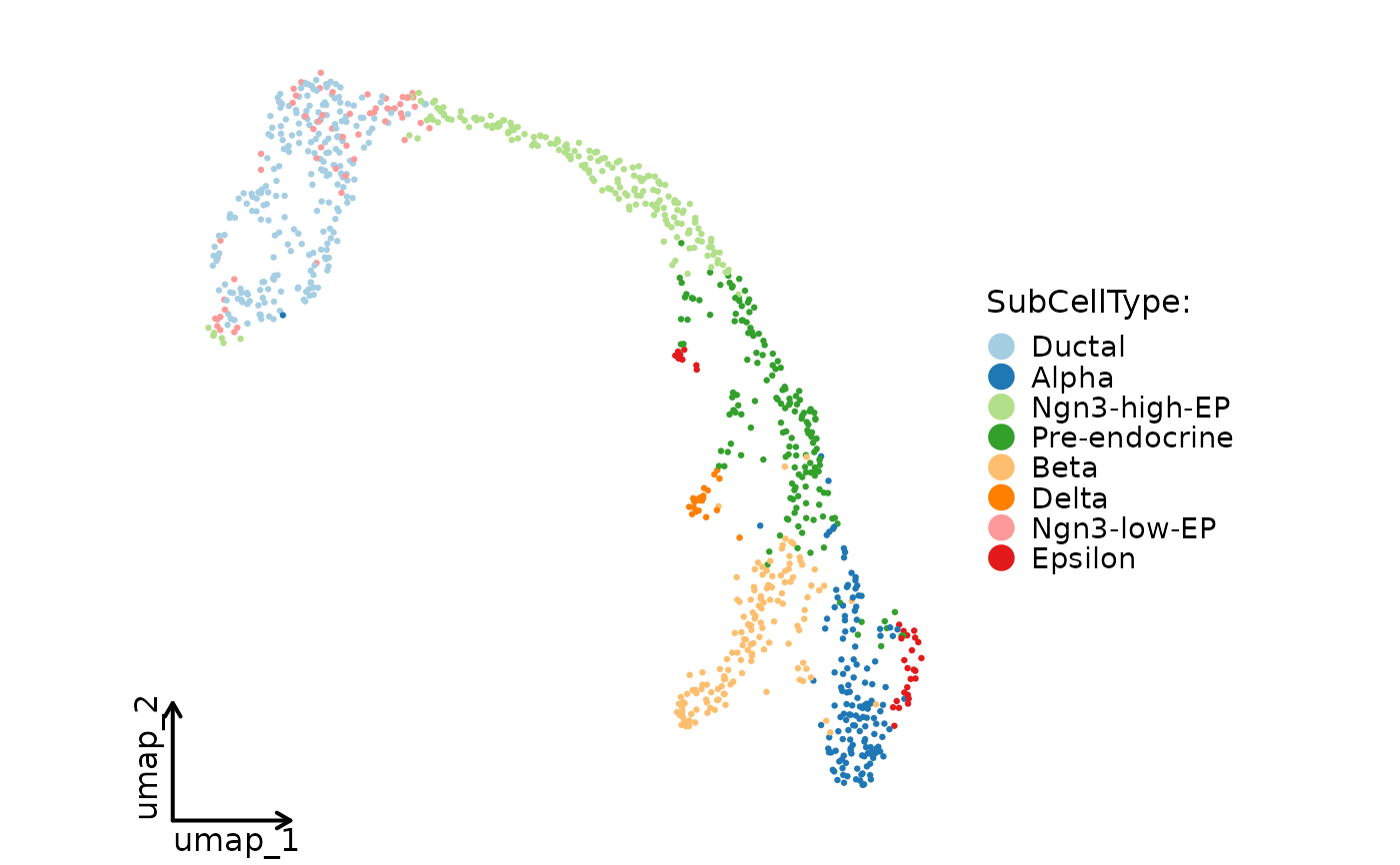
 CellDimPlot(
pancreas_sub,
group.by = "SubCellType",
reduction = "UMAP",
theme_use = "theme_blank"
)
CellDimPlot(
pancreas_sub,
group.by = "SubCellType",
reduction = "UMAP",
theme_use = "theme_blank"
)
 CellDimPlot(
pancreas_sub,
group.by = "SubCellType",
reduction = "UMAP",
theme_use = ggplot2::theme_classic,
theme_args = list(base_size = 16)
)
CellDimPlot(
pancreas_sub,
group.by = "SubCellType",
reduction = "UMAP",
theme_use = ggplot2::theme_classic,
theme_args = list(base_size = 16)
)
 # Highlight cells
CellDimPlot(
pancreas_sub,
group.by = "SubCellType",
reduction = "UMAP",
cells.highlight = colnames(
pancreas_sub
)[pancreas_sub$SubCellType == "Epsilon"]
)
# Highlight cells
CellDimPlot(
pancreas_sub,
group.by = "SubCellType",
reduction = "UMAP",
cells.highlight = colnames(
pancreas_sub
)[pancreas_sub$SubCellType == "Epsilon"]
)
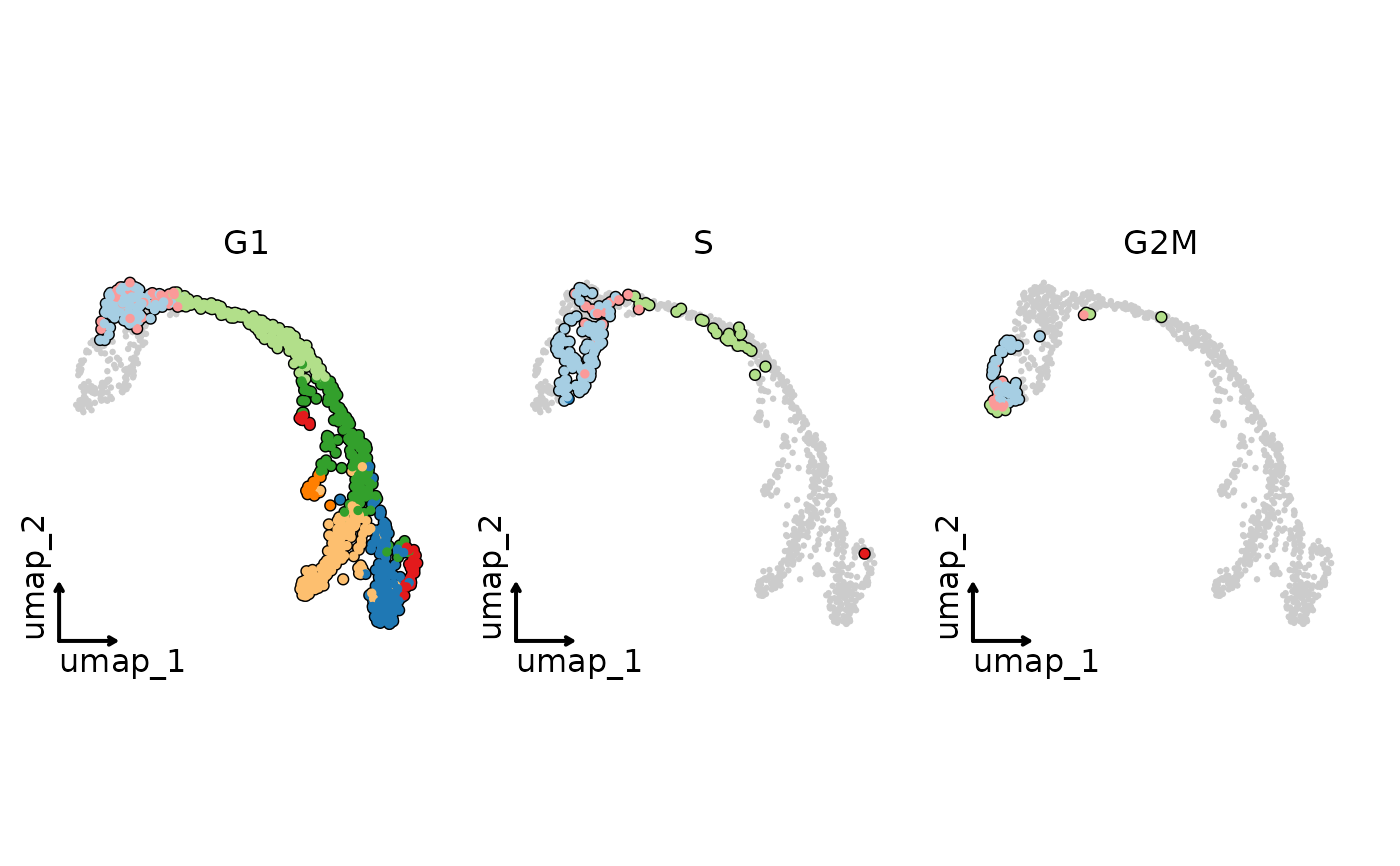
 CellDimPlot(
pancreas_sub,
group.by = "SubCellType",
split.by = "Phase",
reduction = "UMAP",
cells.highlight = TRUE,
theme_use = "theme_blank",
legend.position = "none"
)
CellDimPlot(
pancreas_sub,
group.by = "SubCellType",
split.by = "Phase",
reduction = "UMAP",
cells.highlight = TRUE,
theme_use = "theme_blank",
legend.position = "none"
)
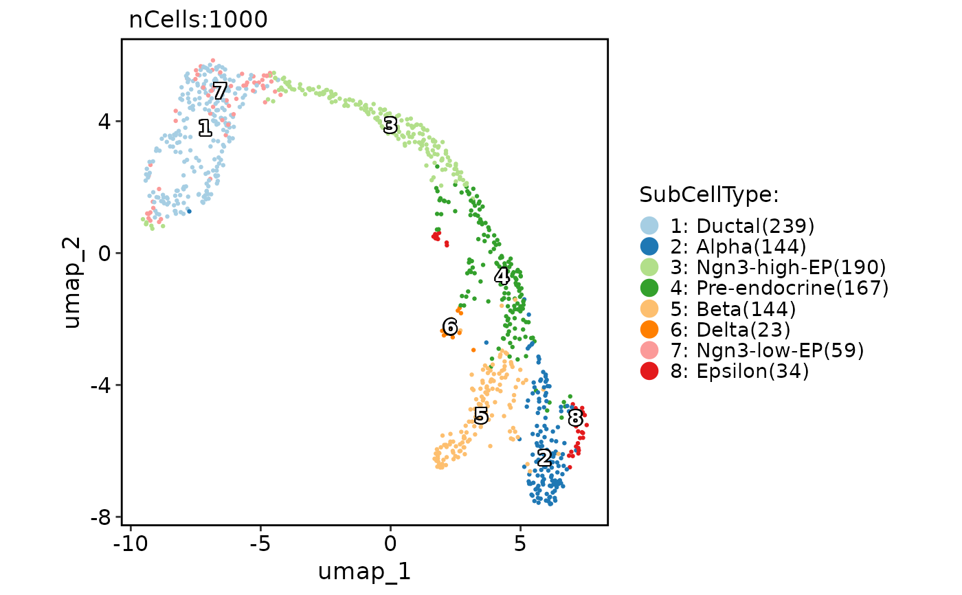
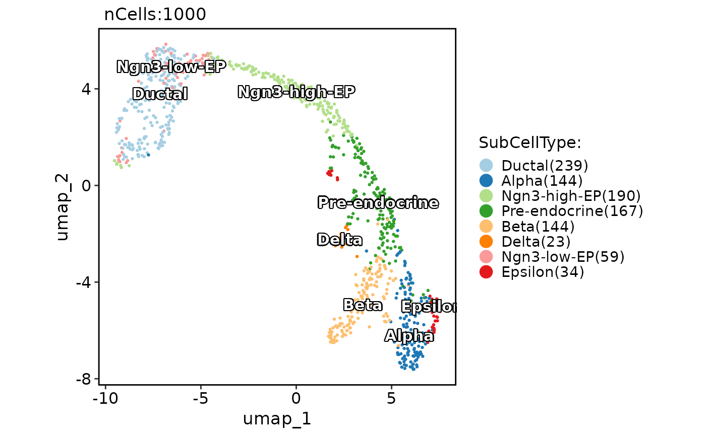
 # Add group labels
CellDimPlot(
pancreas_sub,
group.by = "SubCellType",
reduction = "UMAP",
label = TRUE
)
# Add group labels
CellDimPlot(
pancreas_sub,
group.by = "SubCellType",
reduction = "UMAP",
label = TRUE
)
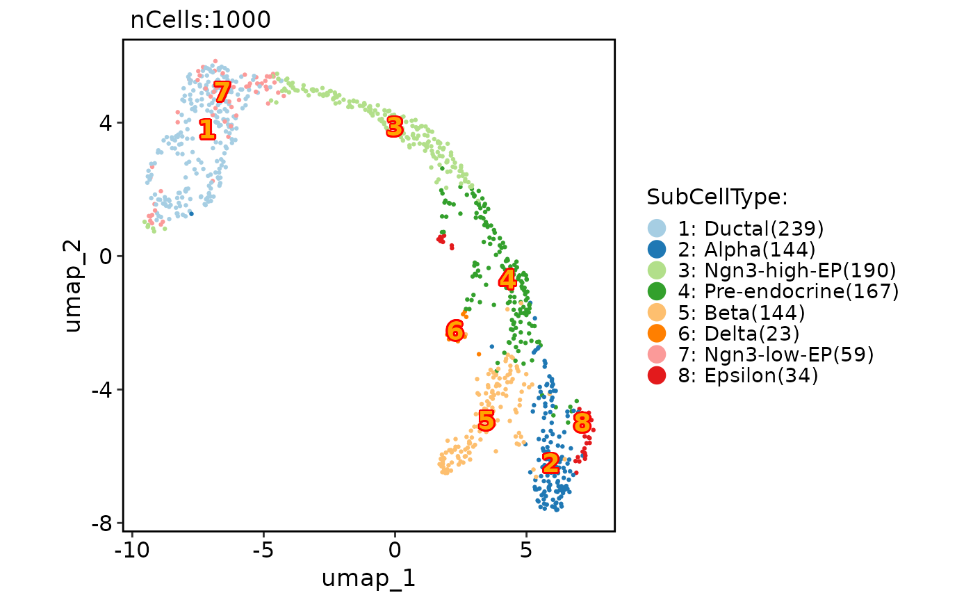
 CellDimPlot(
pancreas_sub,
group.by = "SubCellType",
reduction = "UMAP",
label = TRUE,
label.fg = "orange",
label.bg = "red",
label.size = 5
)
CellDimPlot(
pancreas_sub,
group.by = "SubCellType",
reduction = "UMAP",
label = TRUE,
label.fg = "orange",
label.bg = "red",
label.size = 5
)
 CellDimPlot(
pancreas_sub,
group.by = "SubCellType",
reduction = "UMAP",
label = TRUE,
label_insitu = TRUE
)
CellDimPlot(
pancreas_sub,
group.by = "SubCellType",
reduction = "UMAP",
label = TRUE,
label_insitu = TRUE
)
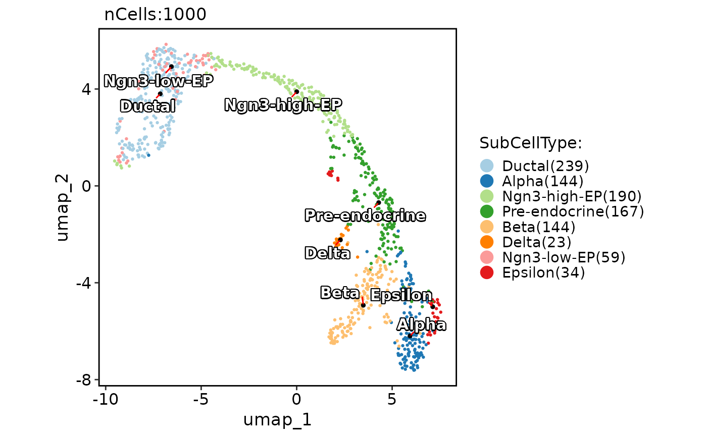
 CellDimPlot(
pancreas_sub,
group.by = "SubCellType",
reduction = "UMAP",
label = TRUE,
label_insitu = TRUE,
label_repel = TRUE,
label_segment_color = "red"
)
CellDimPlot(
pancreas_sub,
group.by = "SubCellType",
reduction = "UMAP",
label = TRUE,
label_insitu = TRUE,
label_repel = TRUE,
label_segment_color = "red"
)
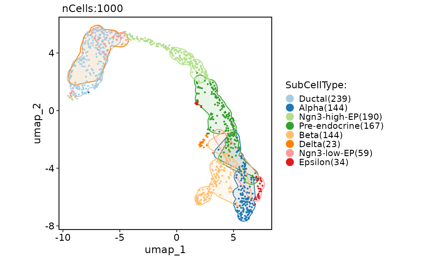
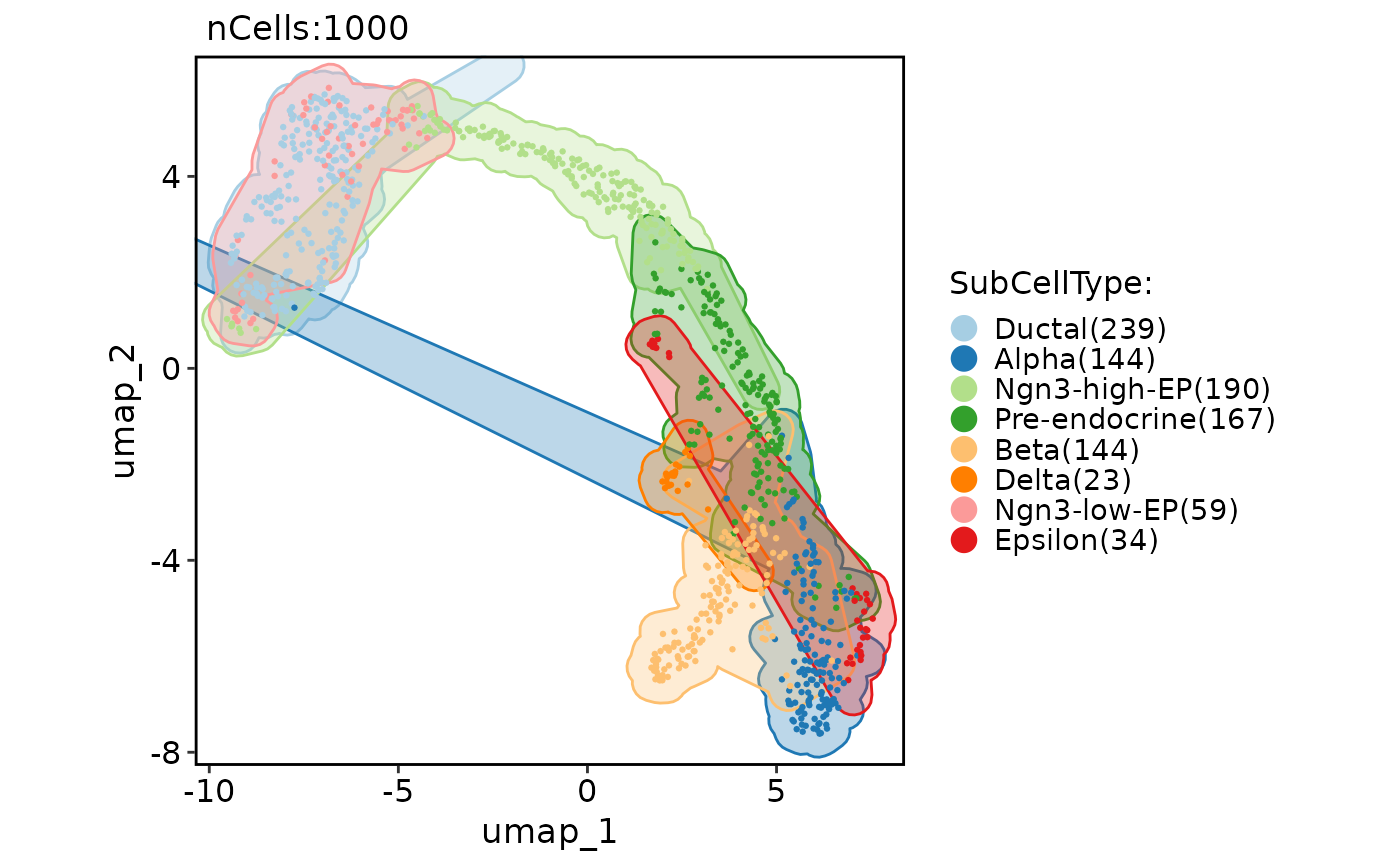
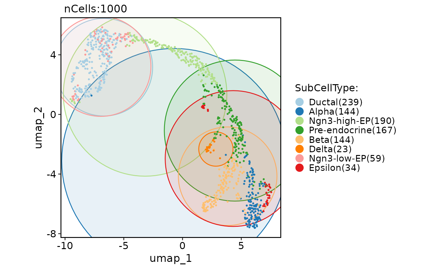
 # Add various shape of marks
CellDimPlot(
pancreas_sub,
group.by = "SubCellType",
reduction = "UMAP",
add_mark = TRUE
)
# Add various shape of marks
CellDimPlot(
pancreas_sub,
group.by = "SubCellType",
reduction = "UMAP",
add_mark = TRUE
)
 CellDimPlot(
pancreas_sub,
group.by = "SubCellType",
reduction = "UMAP",
add_mark = TRUE,
mark_expand = grid::unit(1, "mm")
)
CellDimPlot(
pancreas_sub,
group.by = "SubCellType",
reduction = "UMAP",
add_mark = TRUE,
mark_expand = grid::unit(1, "mm")
)
 CellDimPlot(
pancreas_sub,
group.by = "SubCellType",
reduction = "UMAP",
add_mark = TRUE,
mark_alpha = 0.3
)
CellDimPlot(
pancreas_sub,
group.by = "SubCellType",
reduction = "UMAP",
add_mark = TRUE,
mark_alpha = 0.3
)
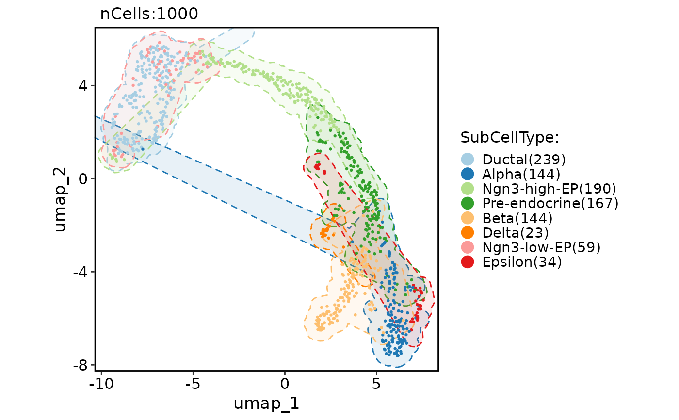
 CellDimPlot(
pancreas_sub,
group.by = "SubCellType",
reduction = "UMAP",
add_mark = TRUE,
mark_linetype = 2
)
CellDimPlot(
pancreas_sub,
group.by = "SubCellType",
reduction = "UMAP",
add_mark = TRUE,
mark_linetype = 2
)
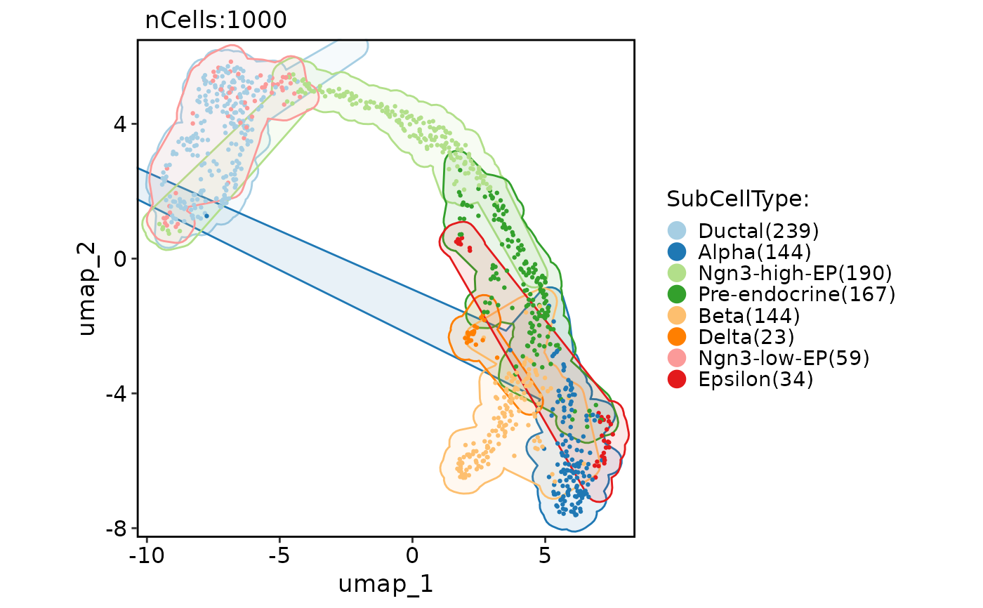
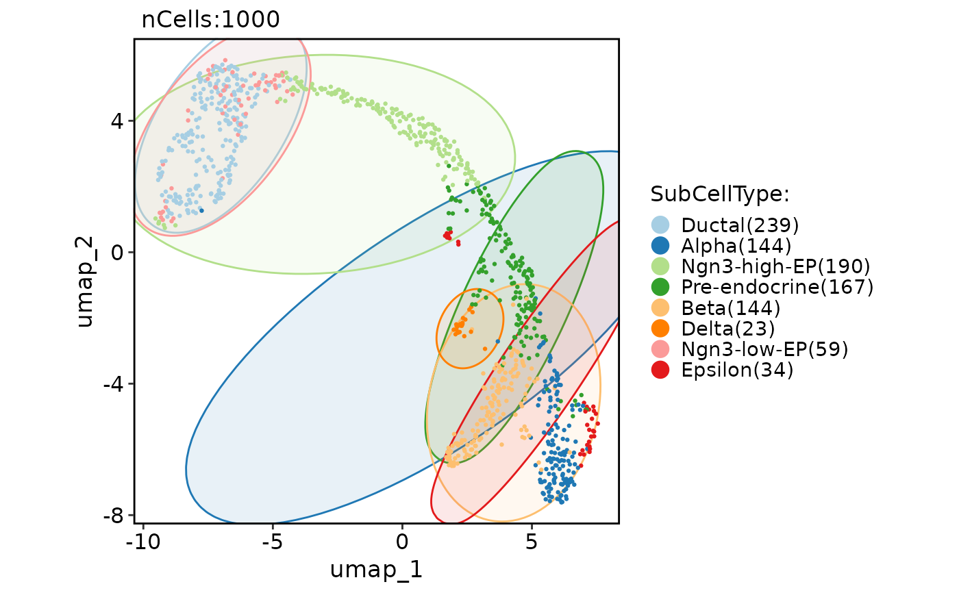
 CellDimPlot(
pancreas_sub,
group.by = "SubCellType",
reduction = "UMAP",
add_mark = TRUE,
mark_type = "ellipse"
)
CellDimPlot(
pancreas_sub,
group.by = "SubCellType",
reduction = "UMAP",
add_mark = TRUE,
mark_type = "ellipse"
)
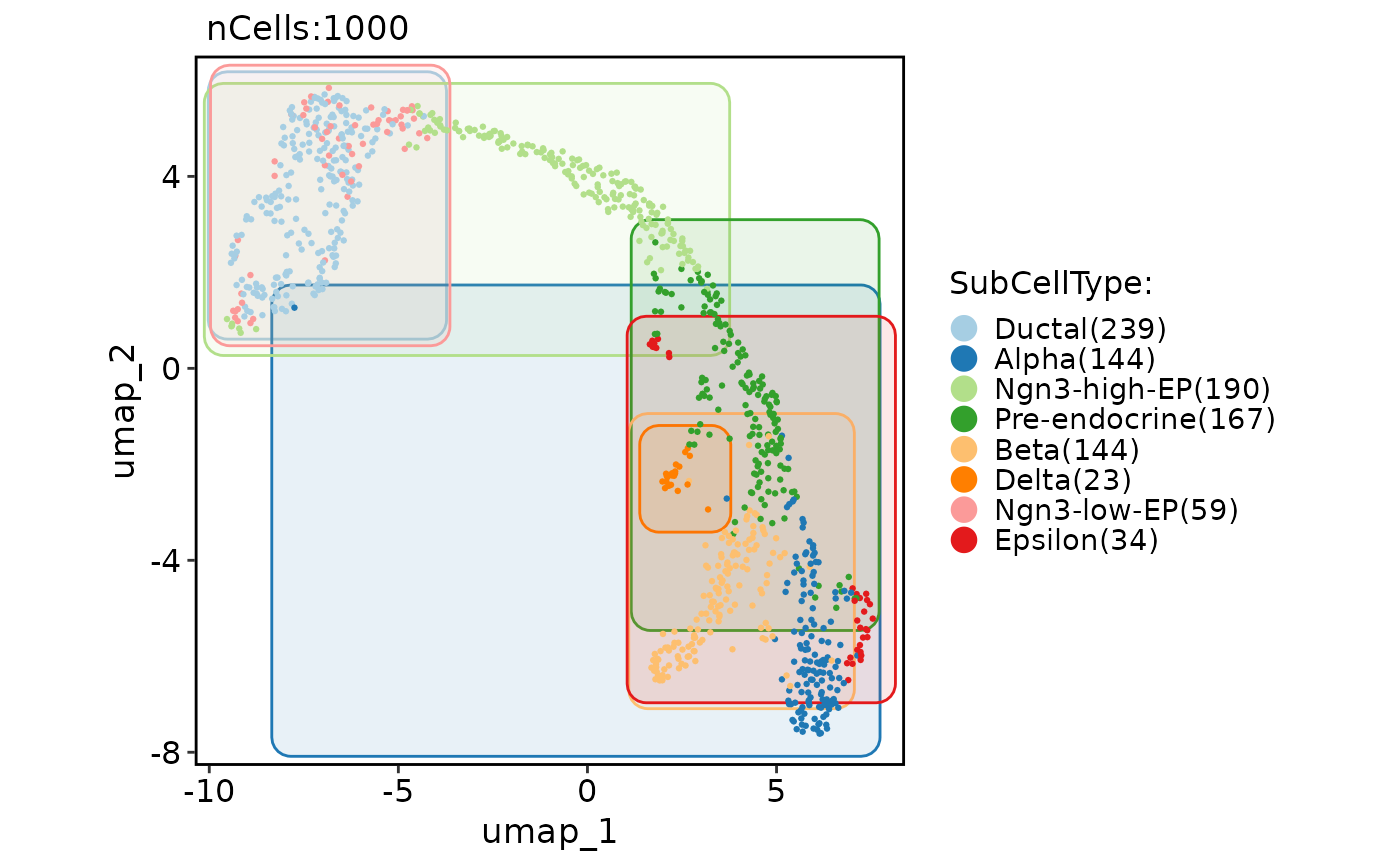
 CellDimPlot(
pancreas_sub,
group.by = "SubCellType",
reduction = "UMAP",
add_mark = TRUE,
mark_type = "rect"
)
CellDimPlot(
pancreas_sub,
group.by = "SubCellType",
reduction = "UMAP",
add_mark = TRUE,
mark_type = "rect"
)
 CellDimPlot(
pancreas_sub,
group.by = "SubCellType",
reduction = "UMAP",
add_mark = TRUE,
mark_type = "circle"
)
CellDimPlot(
pancreas_sub,
group.by = "SubCellType",
reduction = "UMAP",
add_mark = TRUE,
mark_type = "circle"
)
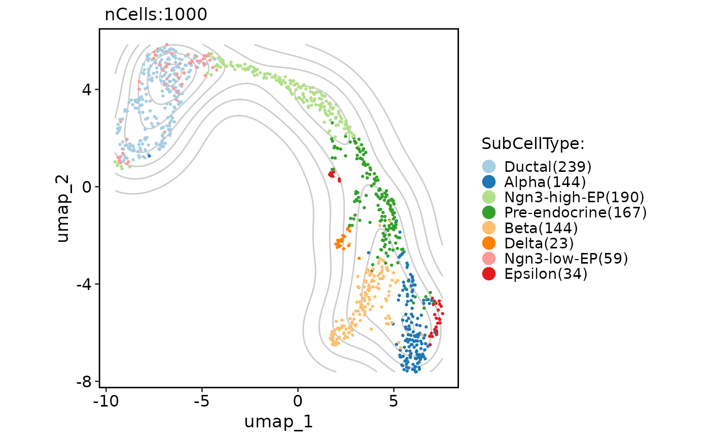
 # Add a density layer
CellDimPlot(
pancreas_sub,
group.by = "SubCellType",
reduction = "UMAP",
add_density = TRUE
)
# Add a density layer
CellDimPlot(
pancreas_sub,
group.by = "SubCellType",
reduction = "UMAP",
add_density = TRUE
)
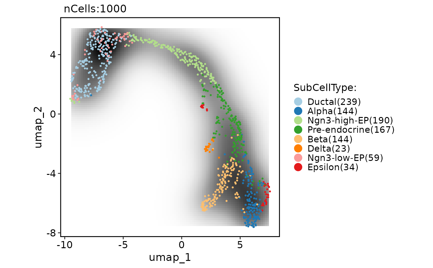
 CellDimPlot(
pancreas_sub,
group.by = "SubCellType",
reduction = "UMAP",
add_density = TRUE,
density_filled = TRUE
)
#> Warning: Removed 396 rows containing missing values or values outside the scale range
#> (`geom_raster()`).
CellDimPlot(
pancreas_sub,
group.by = "SubCellType",
reduction = "UMAP",
add_density = TRUE,
density_filled = TRUE
)
#> Warning: Removed 396 rows containing missing values or values outside the scale range
#> (`geom_raster()`).
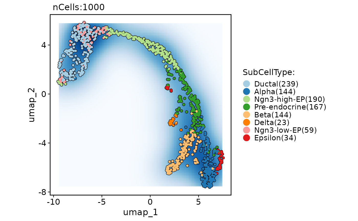
 CellDimPlot(
pancreas_sub,
group.by = "SubCellType",
reduction = "UMAP",
add_density = TRUE,
density_filled = TRUE,
density_filled_palette = "Blues",
cells.highlight = TRUE
)
#> Warning: Removed 396 rows containing missing values or values outside the scale range
#> (`geom_raster()`).
CellDimPlot(
pancreas_sub,
group.by = "SubCellType",
reduction = "UMAP",
add_density = TRUE,
density_filled = TRUE,
density_filled_palette = "Blues",
cells.highlight = TRUE
)
#> Warning: Removed 396 rows containing missing values or values outside the scale range
#> (`geom_raster()`).
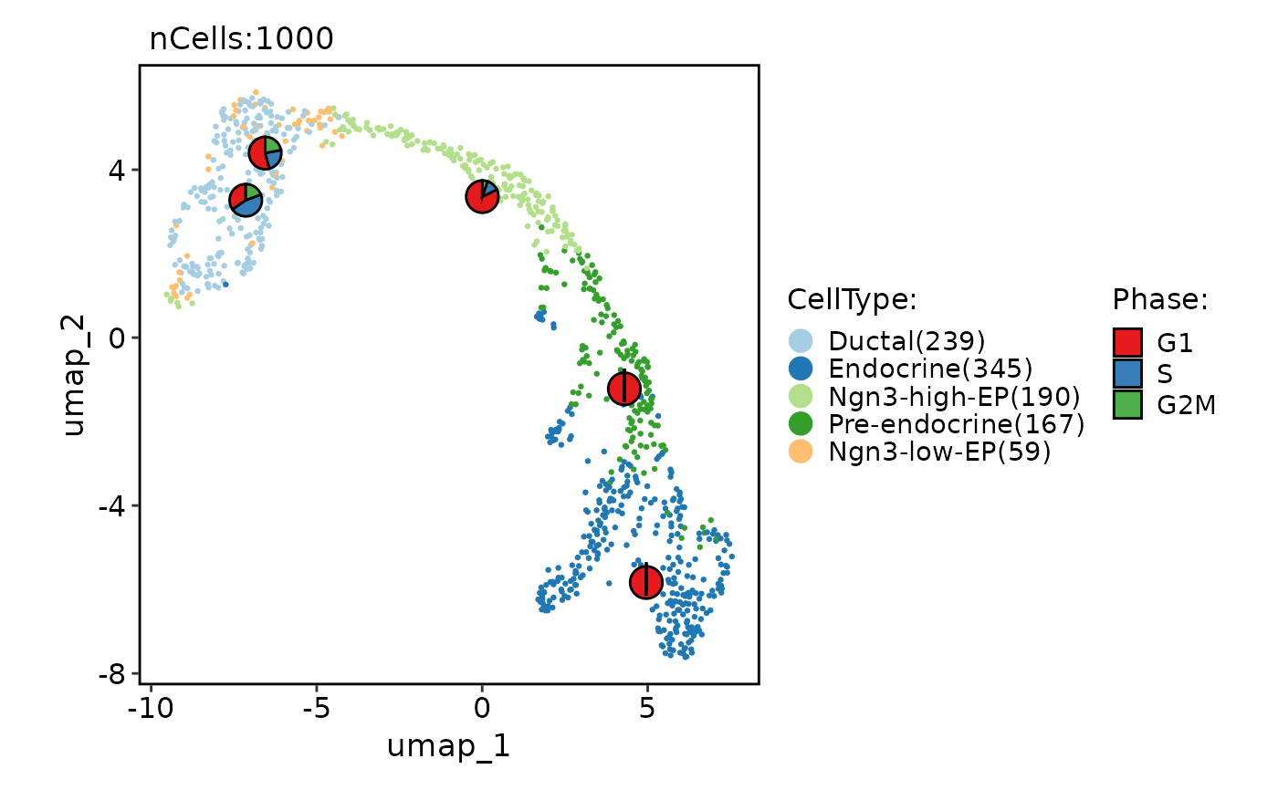
 # Add statistical charts
CellDimPlot(
pancreas_sub,
group.by = "CellType",
reduction = "UMAP",
stat.by = "Phase"
)
# Add statistical charts
CellDimPlot(
pancreas_sub,
group.by = "CellType",
reduction = "UMAP",
stat.by = "Phase"
)
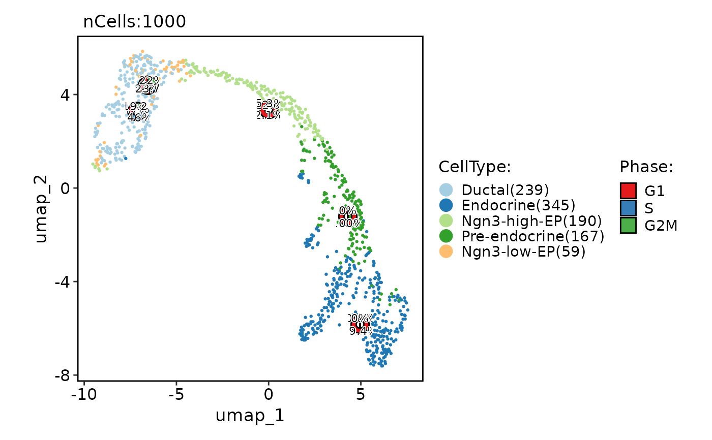
 CellDimPlot(
pancreas_sub,
group.by = "CellType",
reduction = "UMAP",
stat.by = "Phase",
stat_plot_type = "ring",
stat_plot_label = TRUE,
stat_plot_size = 0.15
)
#> Warning: Removed 1 row containing missing values or values outside the scale range
#> (`geom_col()`).
#> Warning: Removed 1 row containing missing values or values outside the scale range
#> (`geom_col()`).
#> Warning: Removed 1 row containing missing values or values outside the scale range
#> (`geom_col()`).
#> Warning: Removed 1 row containing missing values or values outside the scale range
#> (`geom_col()`).
#> Warning: Removed 1 row containing missing values or values outside the scale range
#> (`geom_col()`).
#> Warning: Removed 1 row containing missing values or values outside the scale range
#> (`geom_col()`).
CellDimPlot(
pancreas_sub,
group.by = "CellType",
reduction = "UMAP",
stat.by = "Phase",
stat_plot_type = "ring",
stat_plot_label = TRUE,
stat_plot_size = 0.15
)
#> Warning: Removed 1 row containing missing values or values outside the scale range
#> (`geom_col()`).
#> Warning: Removed 1 row containing missing values or values outside the scale range
#> (`geom_col()`).
#> Warning: Removed 1 row containing missing values or values outside the scale range
#> (`geom_col()`).
#> Warning: Removed 1 row containing missing values or values outside the scale range
#> (`geom_col()`).
#> Warning: Removed 1 row containing missing values or values outside the scale range
#> (`geom_col()`).
#> Warning: Removed 1 row containing missing values or values outside the scale range
#> (`geom_col()`).
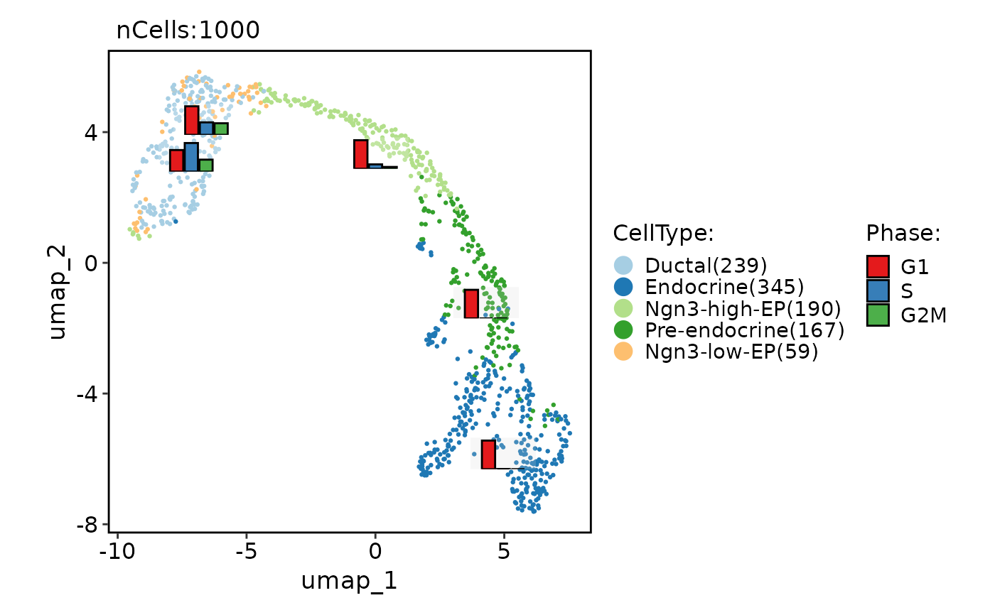
 CellDimPlot(
pancreas_sub,
group.by = "CellType",
reduction = "UMAP",
stat.by = "Phase",
stat_plot_type = "bar",
stat_type = "count",
stat_plot_position = "dodge"
)
CellDimPlot(
pancreas_sub,
group.by = "CellType",
reduction = "UMAP",
stat.by = "Phase",
stat_plot_type = "bar",
stat_type = "count",
stat_plot_position = "dodge"
)
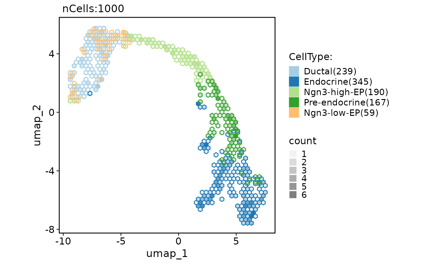
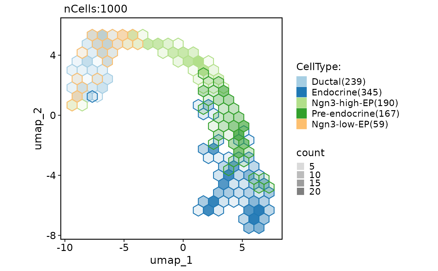
 # Chane the plot type from point to the hexagonal bin
CellDimPlot(
pancreas_sub,
group.by = "CellType",
reduction = "UMAP",
hex = TRUE
)
#> Warning: Removed 7 rows containing missing values or values outside the scale range
#> (`geom_hex()`).
# Chane the plot type from point to the hexagonal bin
CellDimPlot(
pancreas_sub,
group.by = "CellType",
reduction = "UMAP",
hex = TRUE
)
#> Warning: Removed 7 rows containing missing values or values outside the scale range
#> (`geom_hex()`).
 CellDimPlot(
pancreas_sub,
group.by = "CellType",
reduction = "UMAP",
hex = TRUE,
hex.bins = 20
)
#> Warning: Removed 6 rows containing missing values or values outside the scale range
#> (`geom_hex()`).
CellDimPlot(
pancreas_sub,
group.by = "CellType",
reduction = "UMAP",
hex = TRUE,
hex.bins = 20
)
#> Warning: Removed 6 rows containing missing values or values outside the scale range
#> (`geom_hex()`).
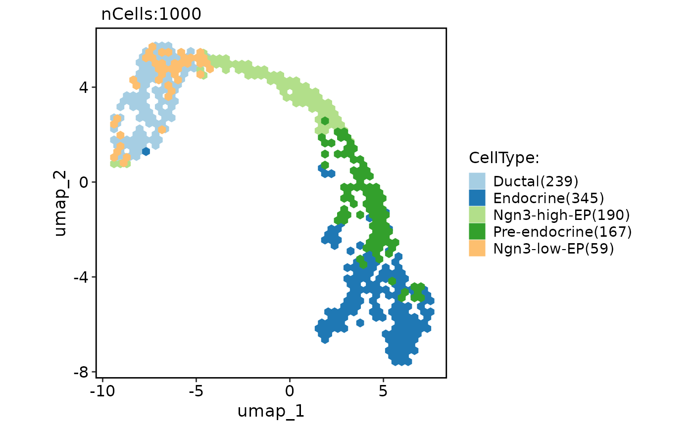
 CellDimPlot(
pancreas_sub,
group.by = "CellType",
reduction = "UMAP",
hex = TRUE,
hex.count = FALSE
)
#> Warning: Removed 7 rows containing missing values or values outside the scale range
#> (`geom_hex()`).
CellDimPlot(
pancreas_sub,
group.by = "CellType",
reduction = "UMAP",
hex = TRUE,
hex.count = FALSE
)
#> Warning: Removed 7 rows containing missing values or values outside the scale range
#> (`geom_hex()`).
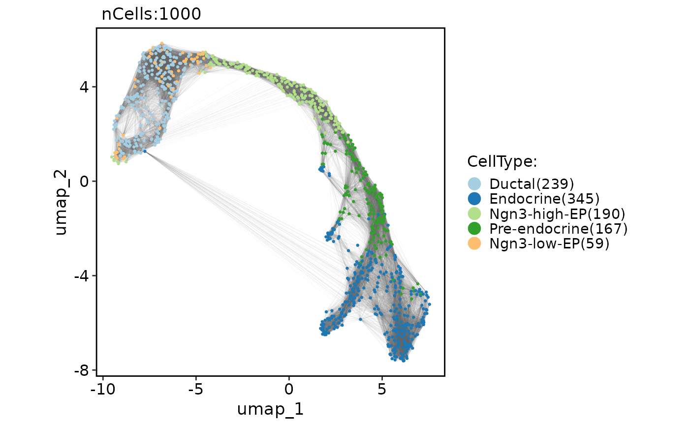
 # Show neighbors graphs on the plot
CellDimPlot(
pancreas_sub,
group.by = "CellType",
reduction = "UMAP",
graph = "Standardpca_SNN"
)
# Show neighbors graphs on the plot
CellDimPlot(
pancreas_sub,
group.by = "CellType",
reduction = "UMAP",
graph = "Standardpca_SNN"
)
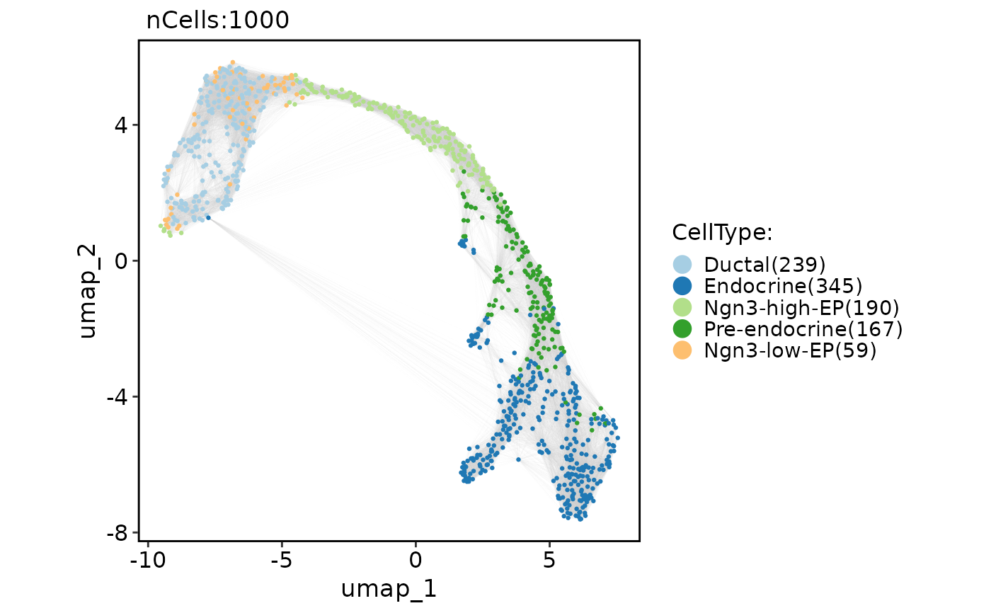
 CellDimPlot(
pancreas_sub,
group.by = "CellType",
reduction = "UMAP",
graph = "Standardpca_SNN",
edge_color = "grey80"
)
CellDimPlot(
pancreas_sub,
group.by = "CellType",
reduction = "UMAP",
graph = "Standardpca_SNN",
edge_color = "grey80"
)
 # Show lineages based on the pseudotime
pancreas_sub <- RunSlingshot(
pancreas_sub,
group.by = "SubCellType",
reduction = "UMAP",
show_plot = FALSE
)
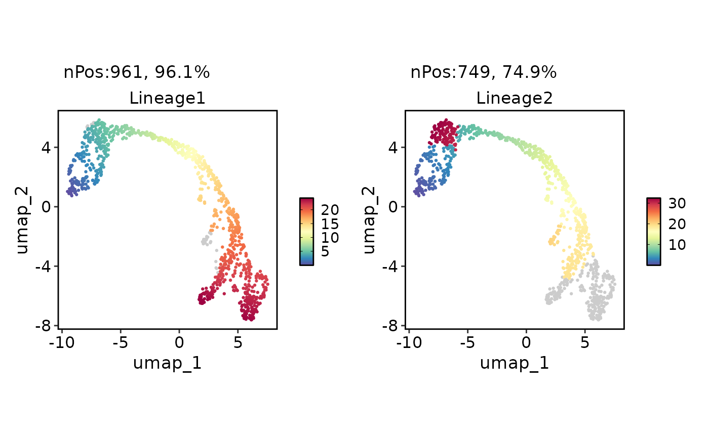
FeatureDimPlot(
pancreas_sub,
features = paste0("Lineage", 1:2),
reduction = "UMAP"
)
# Show lineages based on the pseudotime
pancreas_sub <- RunSlingshot(
pancreas_sub,
group.by = "SubCellType",
reduction = "UMAP",
show_plot = FALSE
)
FeatureDimPlot(
pancreas_sub,
features = paste0("Lineage", 1:2),
reduction = "UMAP"
)
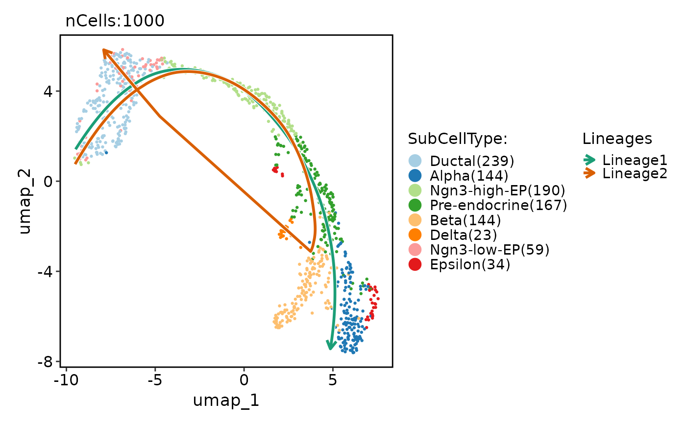
 CellDimPlot(
pancreas_sub,
group.by = "SubCellType",
reduction = "UMAP",
lineages = paste0("Lineage", 1:2)
)
#> Warning: Removed 7 rows containing missing values or values outside the scale range
#> (`geom_path()`).
#> Warning: Removed 7 rows containing missing values or values outside the scale range
#> (`geom_path()`).
CellDimPlot(
pancreas_sub,
group.by = "SubCellType",
reduction = "UMAP",
lineages = paste0("Lineage", 1:2)
)
#> Warning: Removed 7 rows containing missing values or values outside the scale range
#> (`geom_path()`).
#> Warning: Removed 7 rows containing missing values or values outside the scale range
#> (`geom_path()`).
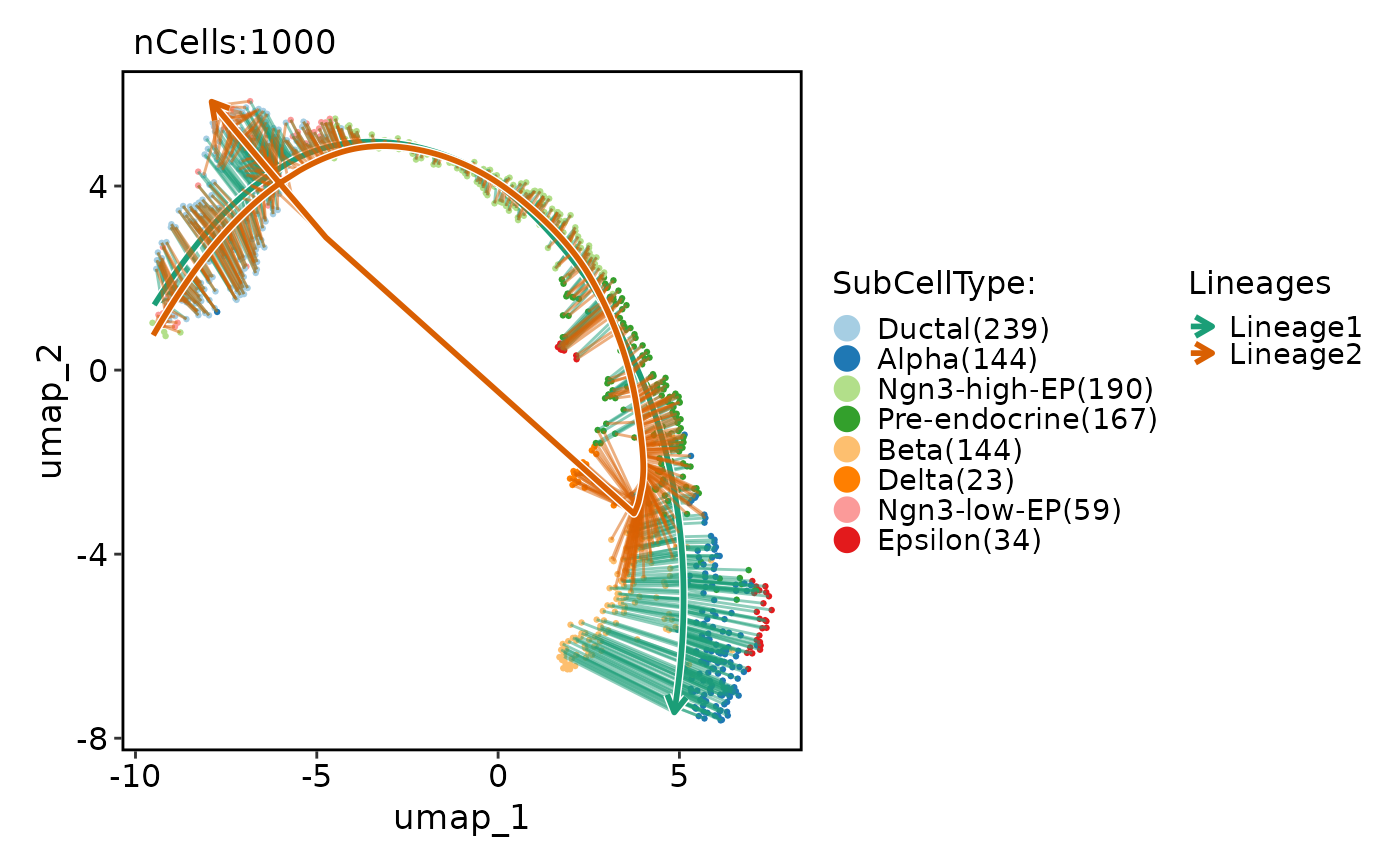
 CellDimPlot(
pancreas_sub,
group.by = "SubCellType",
reduction = "UMAP",
lineages = paste0("Lineage", 1:2),
lineages_whiskers = TRUE
)
#> Warning: Removed 7 rows containing missing values or values outside the scale range
#> (`geom_segment()`).
#> Warning: Removed 7 rows containing missing values or values outside the scale range
#> (`geom_path()`).
#> Warning: Removed 7 rows containing missing values or values outside the scale range
#> (`geom_path()`).
CellDimPlot(
pancreas_sub,
group.by = "SubCellType",
reduction = "UMAP",
lineages = paste0("Lineage", 1:2),
lineages_whiskers = TRUE
)
#> Warning: Removed 7 rows containing missing values or values outside the scale range
#> (`geom_segment()`).
#> Warning: Removed 7 rows containing missing values or values outside the scale range
#> (`geom_path()`).
#> Warning: Removed 7 rows containing missing values or values outside the scale range
#> (`geom_path()`).
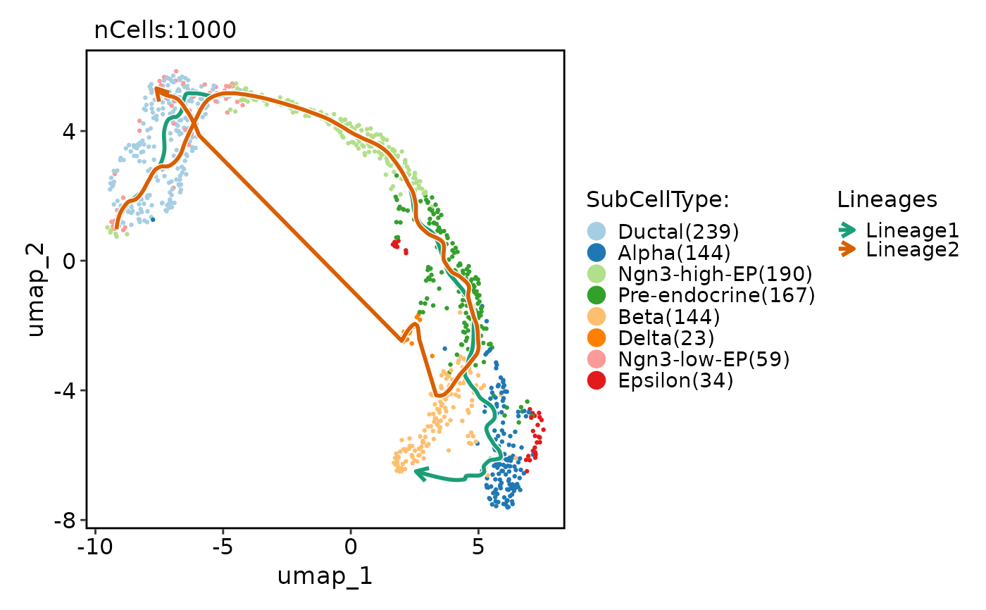
 CellDimPlot(
pancreas_sub,
group.by = "SubCellType",
reduction = "UMAP",
lineages = paste0("Lineage", 1:2),
lineages_span = 0.1
)
CellDimPlot(
pancreas_sub,
group.by = "SubCellType",
reduction = "UMAP",
lineages = paste0("Lineage", 1:2),
lineages_span = 0.1
)
 # Show PAGA results on the plot
pancreas_sub <- RunPAGA(
pancreas_sub,
group.by = "SubCellType",
linear_reduction = "PCA",
nonlinear_reduction = "UMAP",
backend = "cpp",
return_seurat = TRUE
)
#> ℹ [2026-07-22 10:29:53] Running PAGA with BiocNeighbors using 29 neighbors
#> ✔ [2026-07-22 10:29:53] PAGA cpp backend completed
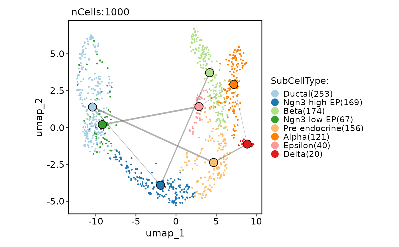
CellDimPlot(
pancreas_sub,
group.by = "SubCellType",
reduction = "UMAP",
paga = pancreas_sub@tools[["PAGA"]]
)
# Show PAGA results on the plot
pancreas_sub <- RunPAGA(
pancreas_sub,
group.by = "SubCellType",
linear_reduction = "PCA",
nonlinear_reduction = "UMAP",
backend = "cpp",
return_seurat = TRUE
)
#> ℹ [2026-07-22 10:29:53] Running PAGA with BiocNeighbors using 29 neighbors
#> ✔ [2026-07-22 10:29:53] PAGA cpp backend completed
CellDimPlot(
pancreas_sub,
group.by = "SubCellType",
reduction = "UMAP",
paga = pancreas_sub@tools[["PAGA"]]
)
 CellDimPlot(
pancreas_sub,
group.by = "SubCellType",
reduction = "UMAP",
paga = pancreas_sub@tools[["PAGA"]],
paga_type = "connectivities_tree"
)
CellDimPlot(
pancreas_sub,
group.by = "SubCellType",
reduction = "UMAP",
paga = pancreas_sub@tools[["PAGA"]],
paga_type = "connectivities_tree"
)
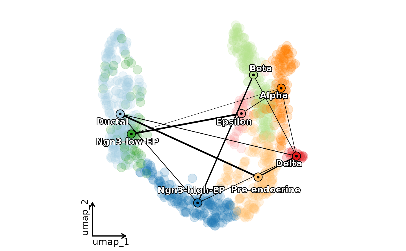
 CellDimPlot(
pancreas_sub,
group.by = "SubCellType",
reduction = "UMAP",
pt.size = 5,
pt.alpha = 0.2,
label = TRUE,
label_repel = TRUE,
label_insitu = TRUE,
label_segment_color = "transparent",
paga = pancreas_sub@tools[["PAGA"]],
paga_edge_threshold = 0.1,
paga_edge_color = "black",
paga_edge_alpha = 1,
legend.position = "none",
theme_use = "theme_blank"
)
CellDimPlot(
pancreas_sub,
group.by = "SubCellType",
reduction = "UMAP",
pt.size = 5,
pt.alpha = 0.2,
label = TRUE,
label_repel = TRUE,
label_insitu = TRUE,
label_segment_color = "transparent",
paga = pancreas_sub@tools[["PAGA"]],
paga_edge_threshold = 0.1,
paga_edge_color = "black",
paga_edge_alpha = 1,
legend.position = "none",
theme_use = "theme_blank"
)
 # Show RNA velocity results on the plot
pancreas_sub <- RunSCVELO(
pancreas_sub,
group.by = "SubCellType",
linear_reduction = "PCA",
nonlinear_reduction = "UMAP",
mode = "stochastic",
backend = "cpp",
return_seurat = TRUE
)
#> ℹ [2026-07-22 10:29:54] Running scanpy-compatible preprocessing (15998 features -> filter + normalize)...
#> ℹ [2026-07-22 10:30:01] Running scVelo "stochastic" mode with `backend = 'cpp'` (10590 features)
#> ✔ [2026-07-22 10:30:15] scVelo "stochastic" mode completed
#> ✔ [2026-07-22 10:30:15] scVelo cpp backend completed
CellDimPlot(
pancreas_sub,
group.by = "SubCellType",
reduction = "UMAP",
velocity = "stochastic"
)
# Show RNA velocity results on the plot
pancreas_sub <- RunSCVELO(
pancreas_sub,
group.by = "SubCellType",
linear_reduction = "PCA",
nonlinear_reduction = "UMAP",
mode = "stochastic",
backend = "cpp",
return_seurat = TRUE
)
#> ℹ [2026-07-22 10:29:54] Running scanpy-compatible preprocessing (15998 features -> filter + normalize)...
#> ℹ [2026-07-22 10:30:01] Running scVelo "stochastic" mode with `backend = 'cpp'` (10590 features)
#> ✔ [2026-07-22 10:30:15] scVelo "stochastic" mode completed
#> ✔ [2026-07-22 10:30:15] scVelo cpp backend completed
CellDimPlot(
pancreas_sub,
group.by = "SubCellType",
reduction = "UMAP",
velocity = "stochastic"
)
 CellDimPlot(
pancreas_sub,
group.by = "SubCellType",
reduction = "UMAP",
pt.size = 5,
pt.alpha = 0.2,
velocity = "stochastic",
velocity_plot_type = "grid"
)
#> Warning: Removed 2 rows containing missing values or values outside the scale range
#> (`geom_segment()`).
CellDimPlot(
pancreas_sub,
group.by = "SubCellType",
reduction = "UMAP",
pt.size = 5,
pt.alpha = 0.2,
velocity = "stochastic",
velocity_plot_type = "grid"
)
#> Warning: Removed 2 rows containing missing values or values outside the scale range
#> (`geom_segment()`).
 CellDimPlot(
pancreas_sub,
group.by = "SubCellType",
reduction = "UMAP",
pt.size = 5,
pt.alpha = 0.2,
velocity = "stochastic",
velocity_plot_type = "grid",
velocity_scale = 1.5
)
#> Warning: Removed 2 rows containing missing values or values outside the scale range
#> (`geom_segment()`).
CellDimPlot(
pancreas_sub,
group.by = "SubCellType",
reduction = "UMAP",
pt.size = 5,
pt.alpha = 0.2,
velocity = "stochastic",
velocity_plot_type = "grid",
velocity_scale = 1.5
)
#> Warning: Removed 2 rows containing missing values or values outside the scale range
#> (`geom_segment()`).
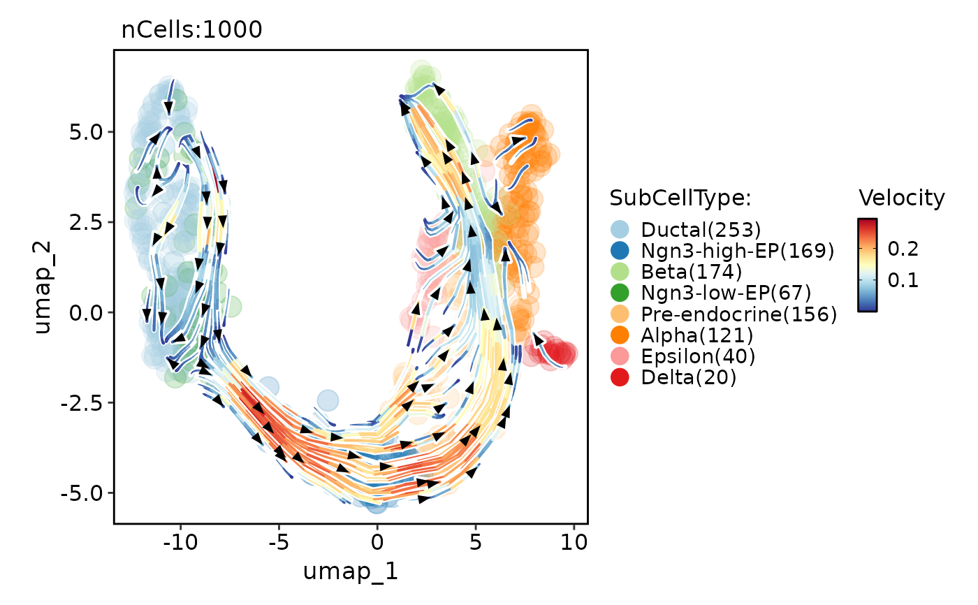
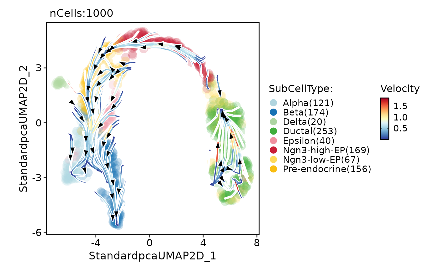
 CellDimPlot(
pancreas_sub,
group.by = "SubCellType",
reduction = "UMAP",
pt.size = 5,
pt.alpha = 0.2,
velocity = "stochastic",
velocity_plot_type = "stream"
)
CellDimPlot(
pancreas_sub,
group.by = "SubCellType",
reduction = "UMAP",
pt.size = 5,
pt.alpha = 0.2,
velocity = "stochastic",
velocity_plot_type = "stream"
)
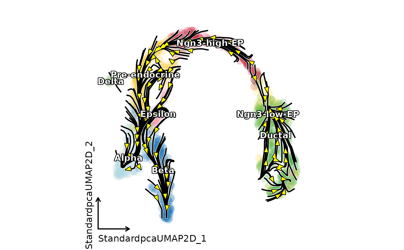
 CellDimPlot(
pancreas_sub,
group.by = "SubCellType",
reduction = "UMAP",
pt.size = 5,
pt.alpha = 0.2,
label = TRUE,
label_insitu = TRUE,
velocity = "stochastic",
velocity_plot_type = "stream",
velocity_arrow_color = "yellow",
velocity_density = 2,
velocity_smooth = 1,
streamline_n = 20,
streamline_color = "black",
legend.position = "none",
theme_use = "theme_blank"
)
CellDimPlot(
pancreas_sub,
group.by = "SubCellType",
reduction = "UMAP",
pt.size = 5,
pt.alpha = 0.2,
label = TRUE,
label_insitu = TRUE,
velocity = "stochastic",
velocity_plot_type = "stream",
velocity_arrow_color = "yellow",
velocity_density = 2,
velocity_smooth = 1,
streamline_n = 20,
streamline_color = "black",
legend.position = "none",
theme_use = "theme_blank"
)