Visualize feature values on a 2-dimensional reduction plot
Source:R/FeatureDimPlot.R
FeatureDimPlot.RdPlotting cell points on a reduced 2D plane and coloring according to the values of the features.
Usage
FeatureDimPlot(
  srt,
  features,
  reduction = NULL,
  dims = c(1, 2),
  split.by = NULL,
  cells = NULL,
  layer = "data",
  assay = NULL,
  show_stat = ifelse(identical(theme_use, "theme_blank"), FALSE, TRUE),
  palette = ifelse(isTRUE(compare_features), "Set1", "Spectral"),
  palcolor = NULL,
  pt.size = NULL,
  pt.alpha = 1,
  bg_cutoff = 0,
  bg_color = "grey80",
  keep_scale = "feature",
  lower_quantile = 0,
  upper_quantile = 0.99,
  lower_cutoff = NULL,
  upper_cutoff = NULL,
  add_density = FALSE,
  density_color = "grey80",
  density_filled = FALSE,
  density_filled_palette = "Greys",
  density_filled_palcolor = NULL,
  cells.highlight = NULL,
  cols.highlight = "black",
  sizes.highlight = 1,
  alpha.highlight = 1,
  stroke.highlight = 0.5,
  calculate_coexp = FALSE,
  compare_features = FALSE,
  color_blend_mode = c("blend", "average", "screen", "multiply"),
  label = FALSE,
  label.size = 4,
  label.fg = "white",
  label.bg = "black",
  label.bg.r = 0.1,
  label_insitu = FALSE,
  label_repel = FALSE,
  label_repulsion = 20,
  label_point_size = 1,
  label_point_color = "black",
  label_segment_color = "black",
  lineages = NULL,
  lineages_trim = c(0.01, 0.99),
  lineages_span = 0.75,
  lineages_palette = "Dark2",
  lineages_palcolor = NULL,
  lineages_arrow = grid::arrow(length = grid::unit(0.1, "inches")),
  lineages_linewidth = 1,
  lineages_line_bg = "white",
  lineages_line_bg_stroke = 0.5,
  lineages_whiskers = FALSE,
  lineages_whiskers_linewidth = 0.5,
  lineages_whiskers_alpha = 0.5,
  graph = NULL,
  edge_size = c(0.05, 0.5),
  edge_alpha = 0.1,
  edge_color = "grey40",
  hex = FALSE,
  hex.linewidth = 0.5,
  hex.color = "grey90",
  hex.bins = 50,
  hex.binwidth = NULL,
  raster = NULL,
  raster.dpi = c(512, 512),
  aspect.ratio = 1,
  title = NULL,
  subtitle = NULL,
  xlab = NULL,
  ylab = NULL,
  legend.position = "right",
  legend.direction = "vertical",
  legend.title = NULL,
  theme_use = "theme_scop",
  theme_args = list(),
  combine = TRUE,
  nrow = NULL,
  ncol = NULL,
  byrow = TRUE,
  force = FALSE,
  seed = 11,
  verbose = TRUE
)
Arguments
- srt
A Seurat object.
- features
A character vector or a named list of features to plot. Features can be gene names in Assay or names of numeric columns in meta.data.
- reduction
Which dimensionality reduction to use. If not specified, will use the reduction returned by DefaultReduction.
- dims
Dimensions to plot, must be a two-length numeric vector specifying x- and y-dimensions
- split.by
Name of a column in meta.data column to split plot by. Default is
NULL.- cells
A character vector of cell names to use.
- layer
Which layer to use. Default is
data.- assay
Which assay to use. If
NULL, the default assay of the Seurat object will be used. When the object also containsChromatinAssay, the default assay and additionalChromatinAssaywill be preprocessed sequentially.- show_stat
Whether to show statistical information on the plot.
- palette
Color palette name. Available palettes can be found in thisplot::show_palettes. Default is
"Chinese".- palcolor
Custom colors used to create a color palette. Default is
NULL.- pt.size
The size of the points in the plot. Default is
NULL, which automatically scales point diameter with the square root of the number of plotted cells.- pt.alpha
The transparency of the data points. Default is
1.- bg_cutoff
Background cutoff. Points with feature values lower than the cutoff will be considered as background and will be colored with
bg_color.- bg_color
Color value for background(NA) points.
- keep_scale
How to handle the color scale across multiple plots. Options are:
NULL(no scaling): Each individual plot is scaled to the maximum expression value of the feature in the condition provided to 'split.by'. Be aware setting NULL will result in color scales that are not comparable between plots."feature"(default; by row/feature scaling): The plots for each individual feature are scaled to the maximum expression of the feature across the conditions provided to 'split.by'."all"(universal scaling): The plots for all features and conditions are scaled to the maximum expression value for the feature with the highest overall expression.
- lower_quantile, upper_quantile, lower_cutoff, upper_cutoff
Vector of minimum and maximum cutoff values or quantile values for each feature.
- add_density
Whether to add a density layer on the plot.
- density_color
Color of the density contours lines.
- density_filled
Whether to add filled contour bands instead of contour lines.
- density_filled_palette
Color palette used to fill contour bands.
- density_filled_palcolor
Custom colors used to fill contour bands.
- cells.highlight
A logical or character vector specifying the cells to highlight in the plot. If
TRUE, all cells are highlighted. IfFALSE, no cells are highlighted. Default isNULL.- cols.highlight
Color used to highlight the cells.
- sizes.highlight
Size of highlighted cell points.
- alpha.highlight
Transparency of highlighted cell points.
- stroke.highlight
Border width of highlighted cell points.
- calculate_coexp
Whether to calculate the co-expression value (geometric mean) of the features.
- compare_features
Whether to show the values of multiple features on a single plot.
- color_blend_mode
Blend mode to use when
compare_features = TRUE- label
Whether the feature name is labeled in the center of the location of cells with high expression.
- label.size
Size of labels.
- label.fg
Foreground color of label.
- label.bg
Background color of label.
- label.bg.r
Background ratio of label.
- label_insitu
Whether the labels is feature names instead of numbers. Valid only when
compare_features = TRUE.- label_repel
Logical value indicating whether the label is repel away from the center points.
- label_repulsion
Force of repulsion between overlapping text labels. Default is
20.- label_point_size
Size of the center points.
- label_point_color
Color of the center points.
- label_segment_color
Color of the line segment for labels.
- lineages
Lineages/pseudotime to add to the plot. If specified, curves will be fitted using stats::loess method.
- lineages_trim
Trim the leading and the trailing data in the lineages.
- lineages_span
The parameter α which controls the degree of smoothing in stats::loess method.
- lineages_palette
Color palette used for lineages.
- lineages_palcolor
Custom colors used for lineages.
- lineages_arrow
Set arrows of the lineages. See grid::arrow.
- lineages_linewidth
Width of fitted curve lines for lineages.
- lineages_line_bg
Background color of curve lines for lineages.
- lineages_line_bg_stroke
Border width of curve lines background.
- lineages_whiskers
Whether to add whiskers for lineages.
- lineages_whiskers_linewidth
Width of whiskers for lineages.
- lineages_whiskers_alpha
Transparency of whiskers for lineages.
- graph
Specify the graph name to add edges between cell neighbors to the plot.
- edge_size
Size of edges.
- edge_alpha
Transparency of edges.
- edge_color
Color of edges.
- hex
Whether to chane the plot type from point to the hexagonal bin.
- hex.linewidth
Border width of hexagonal bins.
- hex.color
Border color of hexagonal bins.
- hex.bins
Number of hexagonal bins.
- hex.binwidth
Hexagonal bin width.
- raster
Convert points to raster format. Default is
NULL, which automatically rasterizes if plotting more than 100,000 cells.- raster.dpi
Pixel resolution for rasterized plots. Default is
c(512, 512).- aspect.ratio
Aspect ratio of the panel. Default is
1.- title
The text for the title. Default is
NULL.- subtitle
The text for the subtitle for the plot which will be displayed below the title. Default is
NULL.- xlab
The x-axis label of the plot. Default is
NULL.- ylab
The y-axis label of the plot. Default is
NULL.- legend.position
The position of legends, one of
"none","left","right","bottom","top". Default is"right".- legend.direction
The direction of the legend in the plot. Can be one of
"vertical"or"horizontal".- legend.title
Title for the legend. Default is
NULL, which uses the group name.- theme_use
Theme used. Can be a character string or a theme function. Default is
"theme_scop".- theme_args
Other arguments passed to the
theme_use. Default islist().- combine
Combine plots into a single
patchworkobject. IfFALSE, return a list of ggplot objects.- nrow
Number of rows in the combined plot. Default is
NULL, which means determined automatically based on the number of plots.- ncol
Number of columns in the combined plot. Default is
NULL, which means determined automatically based on the number of plots.- byrow
Whether to arrange the plots by row in the combined plot. Default is
TRUE.- force
Whether to force drawing regardless of the number of features greater than 100. Default is
FALSE.- seed
Random seed for reproducibility. Default is
11.- verbose
Whether to print the message. Default is
TRUE.
Examples
data(pancreas_sub)
pancreas_sub <- standard_scop(pancreas_sub)
#> ℹ [2026-07-22 10:30:32] Start standard processing workflow...
#> ℹ [2026-07-22 10:30:32] Checking a list of <Seurat>...
#> ! [2026-07-22 10:30:33] Data 1/1 of the `srt_list` is "unknown"
#> ℹ [2026-07-22 10:30:33] Perform `NormalizeData()` with `normalization.method = 'LogNormalize'` on 1/1 of `srt_list`...
#> ℹ [2026-07-22 10:30:33] Perform `FindVariableFeatures()` on 1/1 of `srt_list`...
#> ℹ [2026-07-22 10:30:33] Use the separate HVF from `srt_list`
#> ℹ [2026-07-22 10:30:33] Number of available HVF: 2000
#> ℹ [2026-07-22 10:30:33] Finished check
#> ℹ [2026-07-22 10:30:33] Perform `ScaleData()`
#> ℹ [2026-07-22 10:30:33] Perform pca linear dimension reduction
#> ℹ [2026-07-22 10:30:34] Use stored estimated dimensions 1:23 for Standardpca
#> ℹ [2026-07-22 10:30:35] Perform `Seurat::FindClusters()` with `cluster_algorithm = 'louvain'` and `cluster_resolution = 0.6`
#> ℹ [2026-07-22 10:30:35] Reorder clusters...
#> ℹ [2026-07-22 10:30:35] Skip `log1p()` because `layer = data` is not "counts"
#> ℹ [2026-07-22 10:30:35] Perform umap nonlinear dimension reduction
#> ✔ [2026-07-22 10:30:41] Standard processing workflow completed
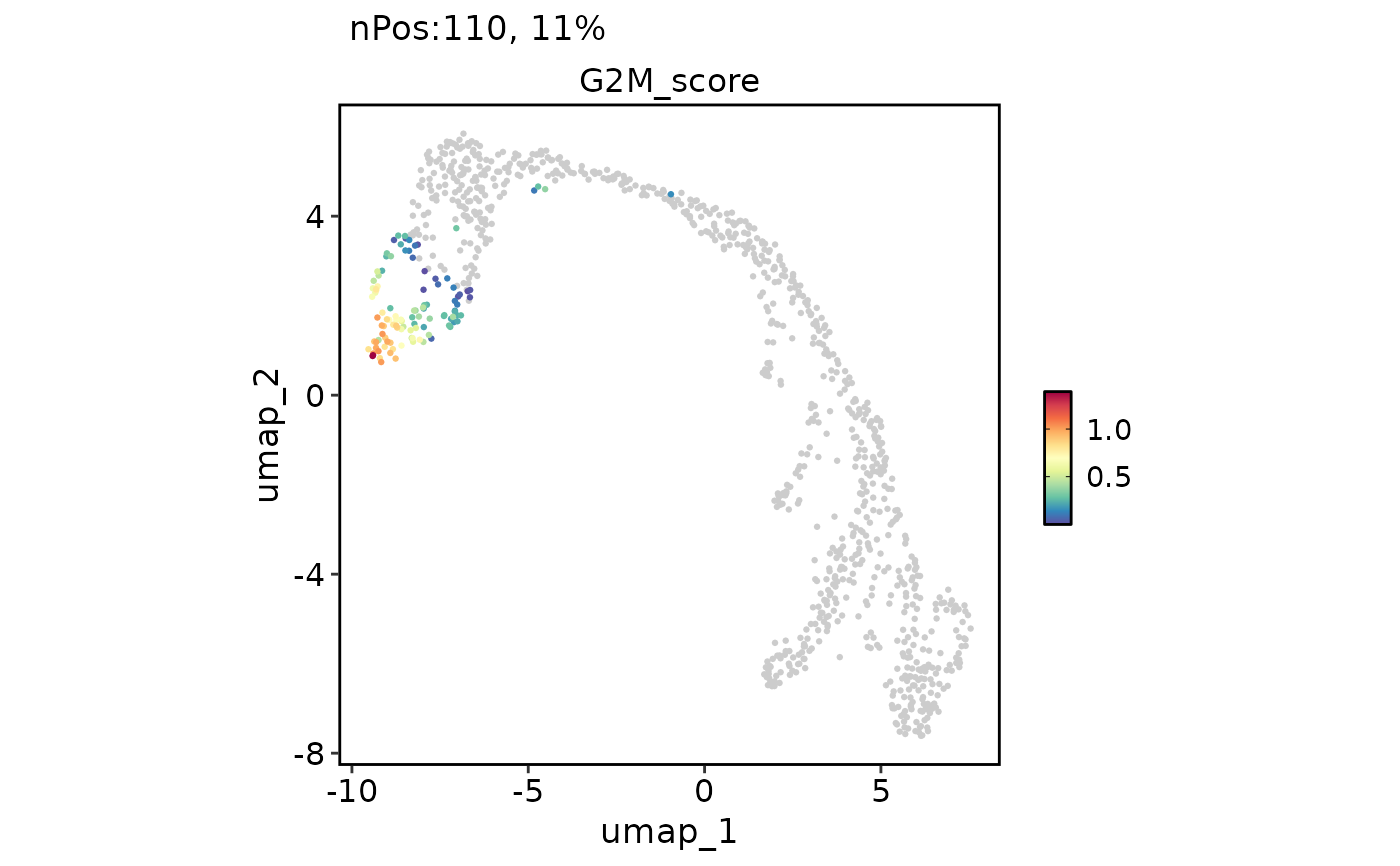
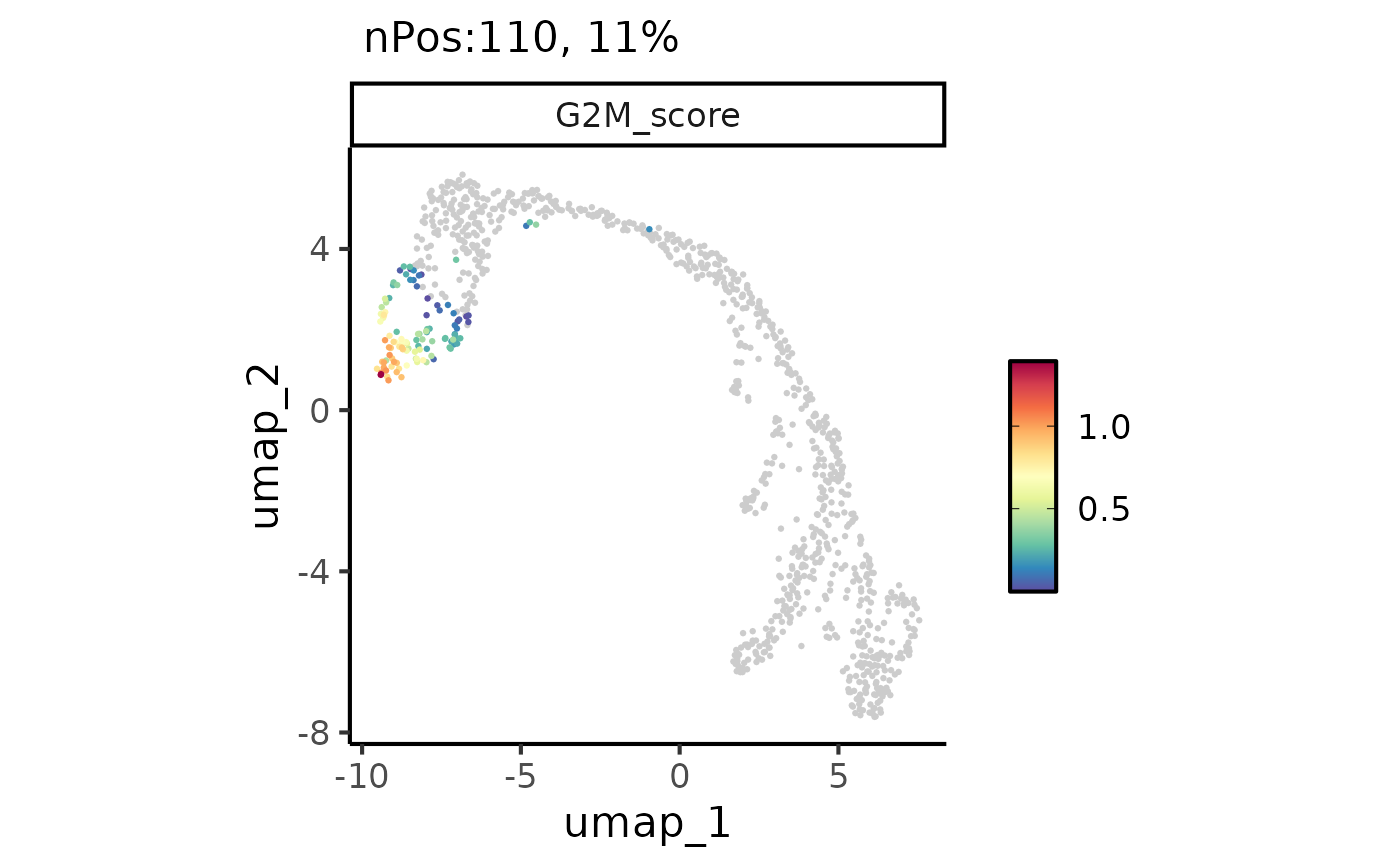
FeatureDimPlot(
pancreas_sub,
features = "G2M_score", reduction = "UMAP"
)
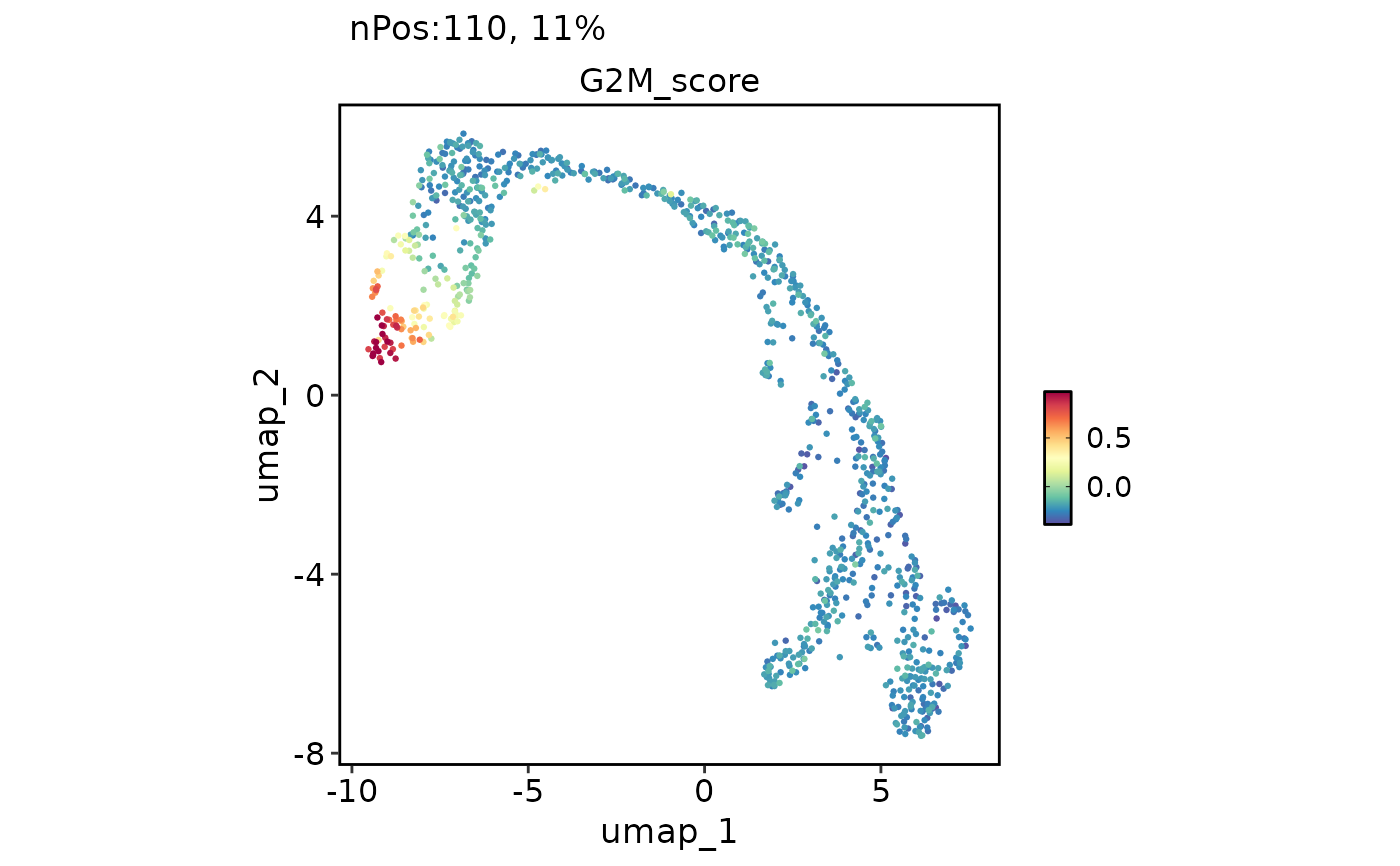
 FeatureDimPlot(
pancreas_sub,
features = "G2M_score",
reduction = "UMAP",
bg_cutoff = -Inf
)
FeatureDimPlot(
pancreas_sub,
features = "G2M_score",
reduction = "UMAP",
bg_cutoff = -Inf
)
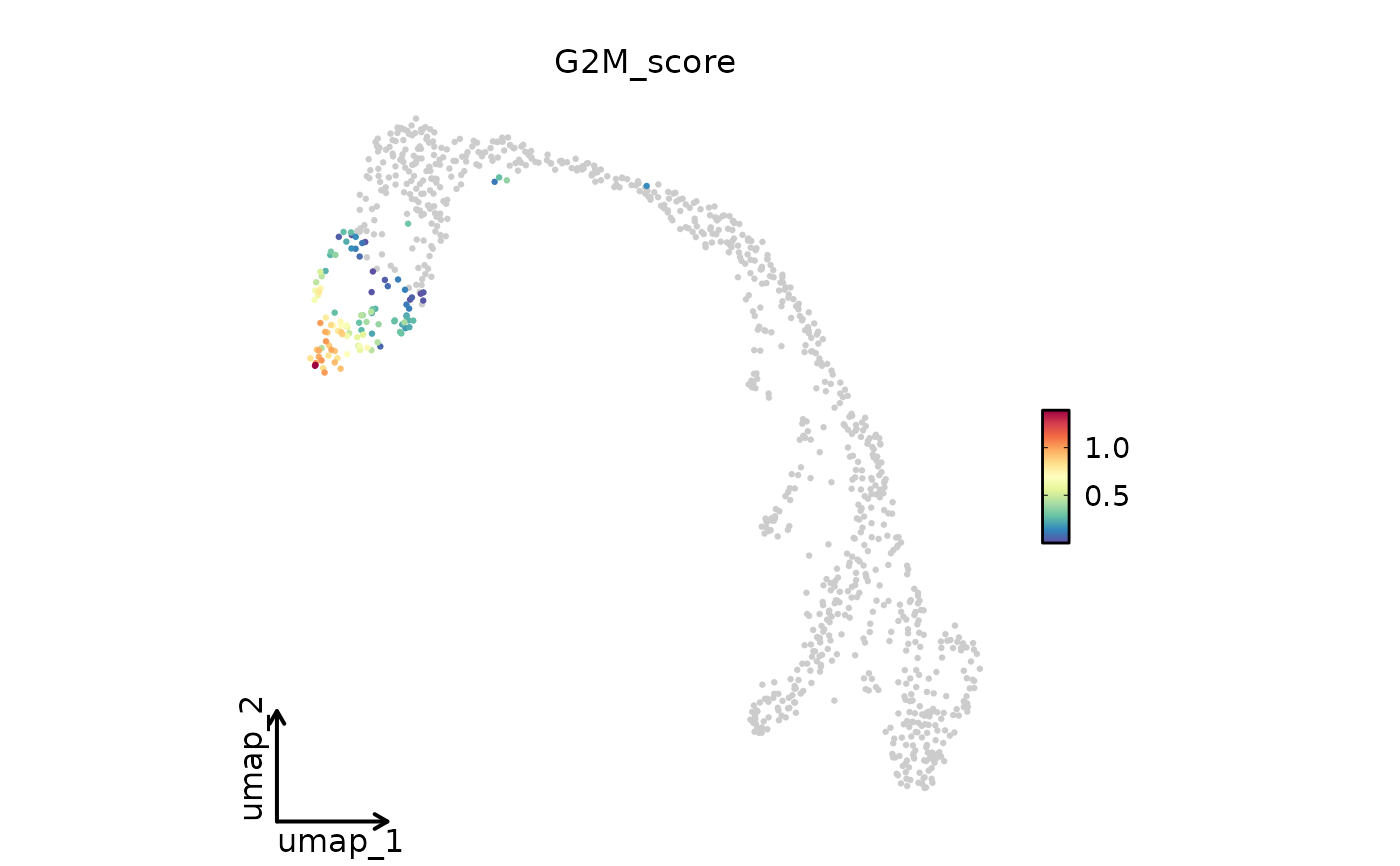
 FeatureDimPlot(
pancreas_sub,
features = "G2M_score",
reduction = "UMAP",
theme_use = "theme_blank"
)
FeatureDimPlot(
pancreas_sub,
features = "G2M_score",
reduction = "UMAP",
theme_use = "theme_blank"
)
 FeatureDimPlot(
pancreas_sub,
features = "G2M_score",
reduction = "UMAP",
theme_use = ggplot2::theme_classic,
theme_args = list(base_size = 16)
)
FeatureDimPlot(
pancreas_sub,
features = "G2M_score",
reduction = "UMAP",
theme_use = ggplot2::theme_classic,
theme_args = list(base_size = 16)
)
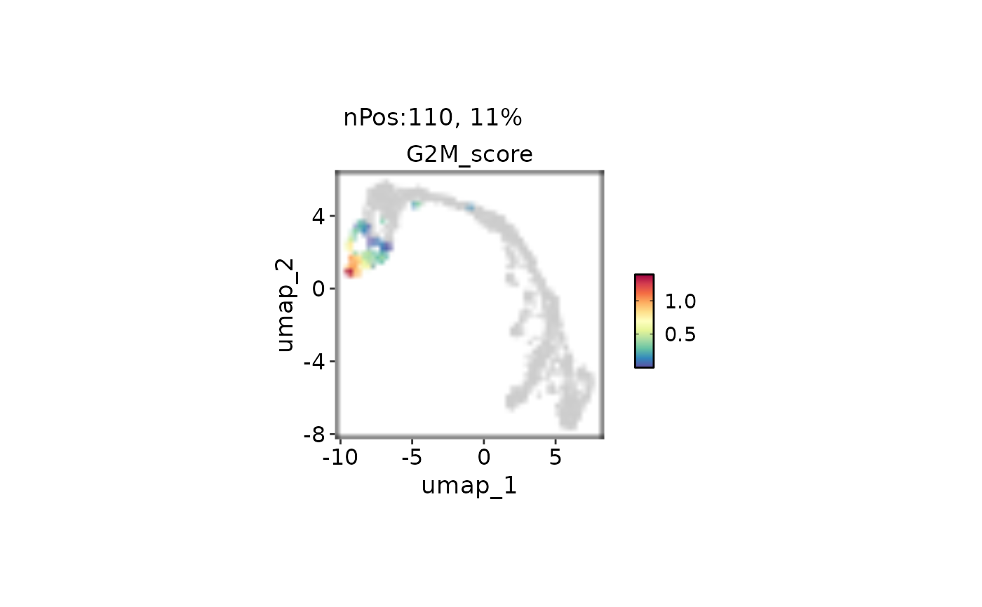
 FeatureDimPlot(
pancreas_sub,
features = "G2M_score",
reduction = "UMAP"
) |> thisplot::panel_fix(
height = 2,
raster = TRUE,
dpi = 30
)
FeatureDimPlot(
pancreas_sub,
features = "G2M_score",
reduction = "UMAP"
) |> thisplot::panel_fix(
height = 2,
raster = TRUE,
dpi = 30
)
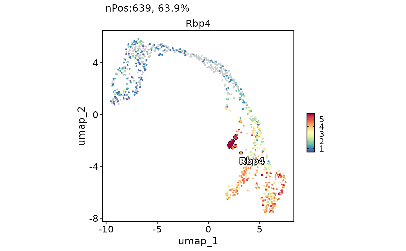
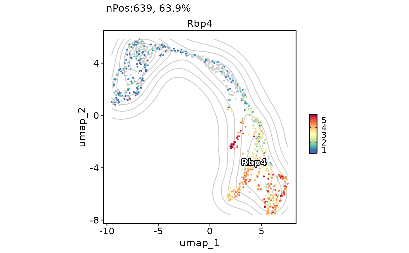
 # Label and highlight cell points
FeatureDimPlot(
pancreas_sub,
features = "Rbp4",
reduction = "UMAP",
label = TRUE,
cells.highlight = colnames(
pancreas_sub
)[pancreas_sub$SubCellType == "Delta"]
)
# Label and highlight cell points
FeatureDimPlot(
pancreas_sub,
features = "Rbp4",
reduction = "UMAP",
label = TRUE,
cells.highlight = colnames(
pancreas_sub
)[pancreas_sub$SubCellType == "Delta"]
)
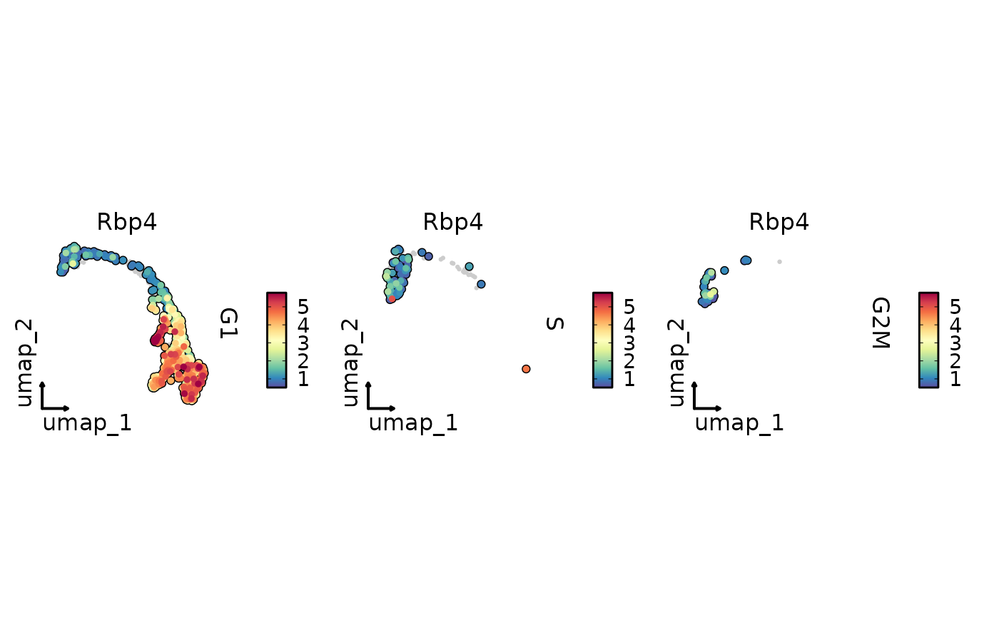
 FeatureDimPlot(
pancreas_sub,
features = "Rbp4",
split.by = "Phase",
reduction = "UMAP",
cells.highlight = TRUE,
theme_use = "theme_blank"
)
FeatureDimPlot(
pancreas_sub,
features = "Rbp4",
split.by = "Phase",
reduction = "UMAP",
cells.highlight = TRUE,
theme_use = "theme_blank"
)
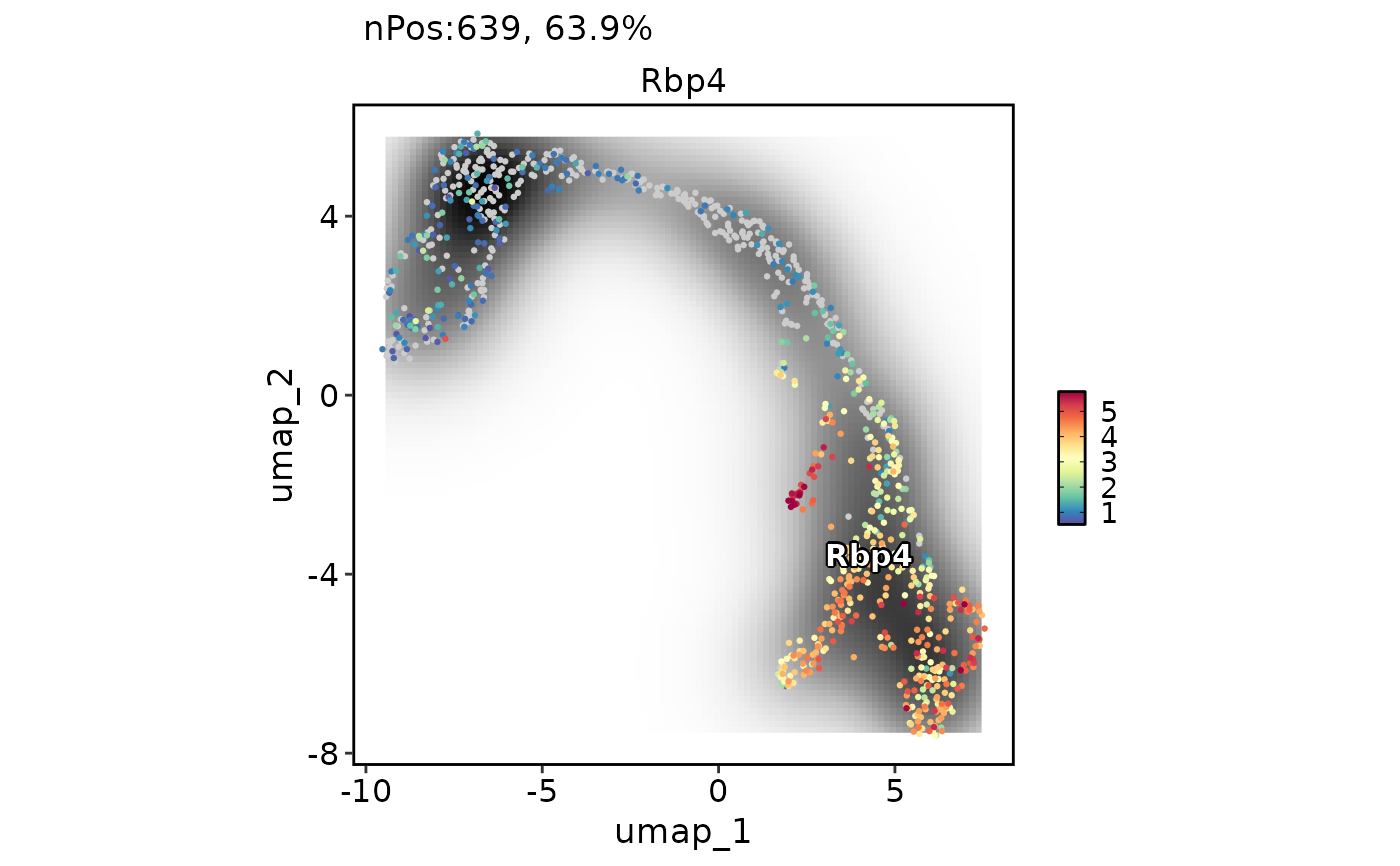
 # Add a density layer
FeatureDimPlot(
pancreas_sub,
features = "Rbp4",
reduction = "UMAP",
label = TRUE,
add_density = TRUE
)
# Add a density layer
FeatureDimPlot(
pancreas_sub,
features = "Rbp4",
reduction = "UMAP",
label = TRUE,
add_density = TRUE
)
 FeatureDimPlot(
pancreas_sub,
features = "Rbp4",
reduction = "UMAP",
label = TRUE,
add_density = TRUE,
density_filled = TRUE
)
#> Warning: Removed 396 rows containing missing values or values outside the scale range
#> (`geom_raster()`).
FeatureDimPlot(
pancreas_sub,
features = "Rbp4",
reduction = "UMAP",
label = TRUE,
add_density = TRUE,
density_filled = TRUE
)
#> Warning: Removed 396 rows containing missing values or values outside the scale range
#> (`geom_raster()`).
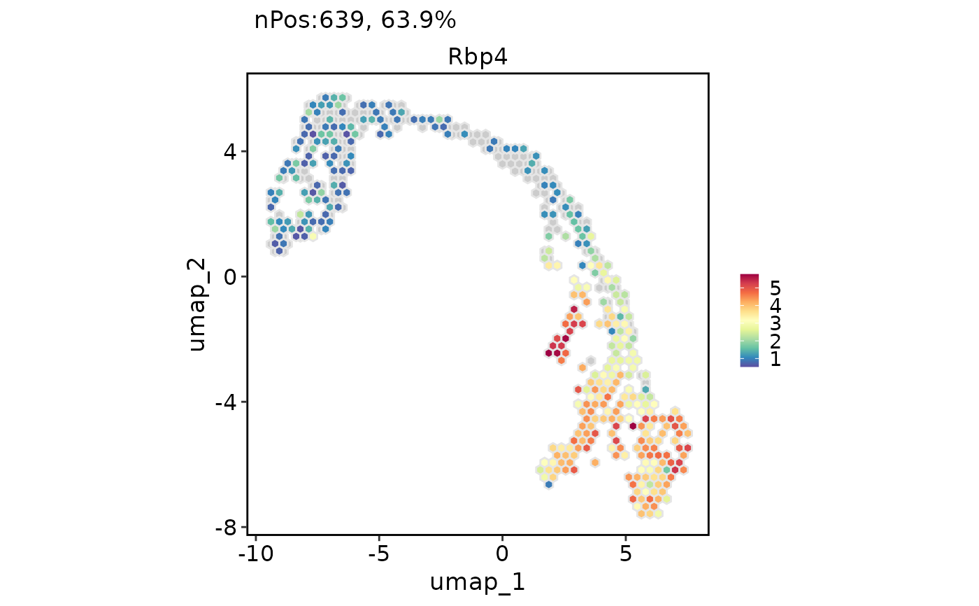
 # Chane the plot type from point to the hexagonal bin
FeatureDimPlot(
pancreas_sub,
features = "Rbp4",
reduction = "UMAP",
hex = TRUE
)
#> Warning: Removed 4 rows containing missing values or values outside the scale range
#> (`geom_hex()`).
#> Warning: Removed 3 rows containing missing values or values outside the scale range
#> (`geom_hex()`).
# Chane the plot type from point to the hexagonal bin
FeatureDimPlot(
pancreas_sub,
features = "Rbp4",
reduction = "UMAP",
hex = TRUE
)
#> Warning: Removed 4 rows containing missing values or values outside the scale range
#> (`geom_hex()`).
#> Warning: Removed 3 rows containing missing values or values outside the scale range
#> (`geom_hex()`).
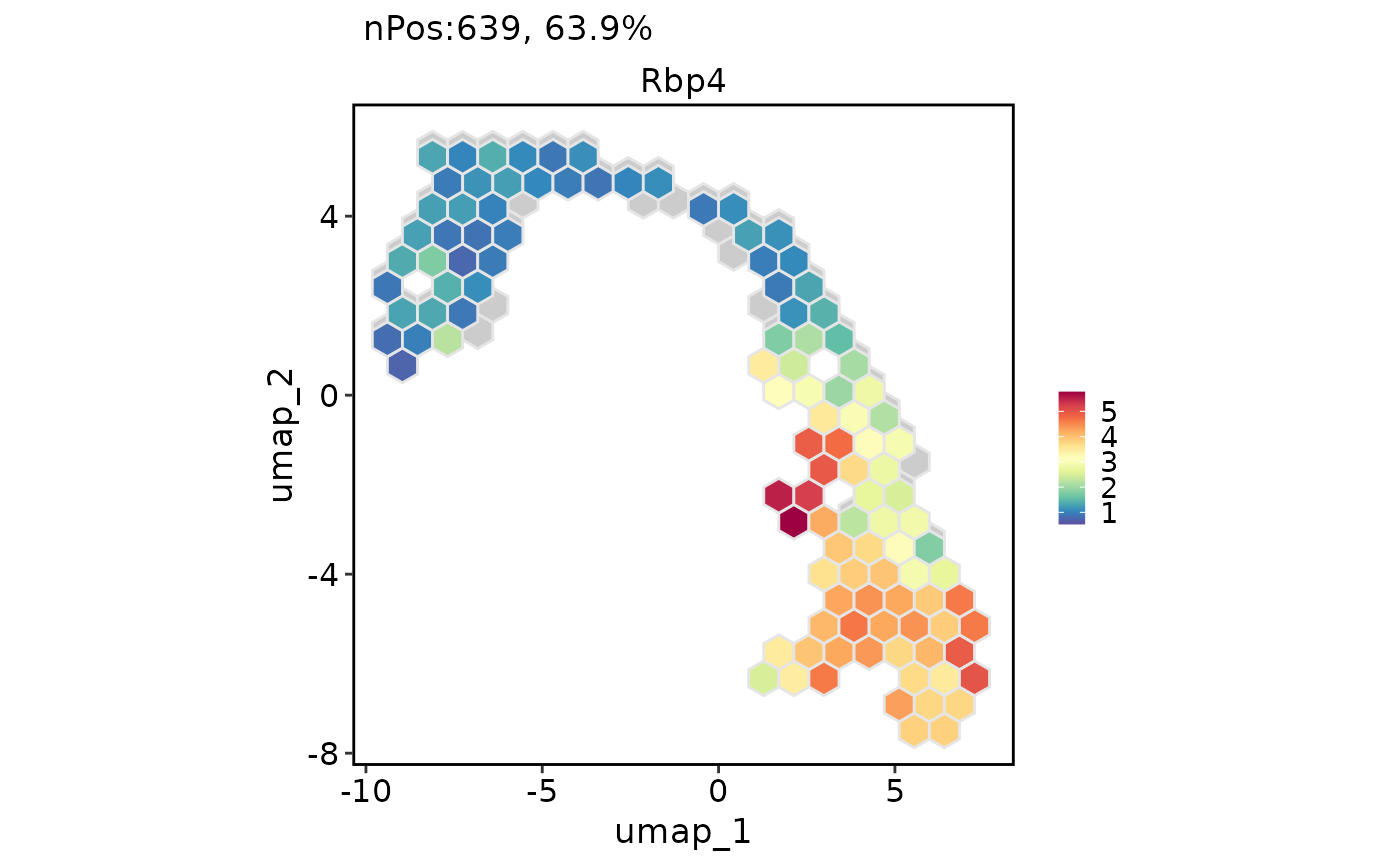
 FeatureDimPlot(
pancreas_sub,
features = "Rbp4",
reduction = "UMAP",
hex = TRUE,
hex.bins = 20
)
#> Warning: Removed 3 rows containing missing values or values outside the scale range
#> (`geom_hex()`).
#> Warning: Removed 3 rows containing missing values or values outside the scale range
#> (`geom_hex()`).
FeatureDimPlot(
pancreas_sub,
features = "Rbp4",
reduction = "UMAP",
hex = TRUE,
hex.bins = 20
)
#> Warning: Removed 3 rows containing missing values or values outside the scale range
#> (`geom_hex()`).
#> Warning: Removed 3 rows containing missing values or values outside the scale range
#> (`geom_hex()`).
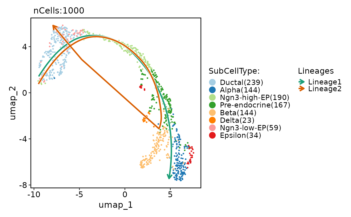
 # Show lineages on the plot based on the pseudotime
pancreas_sub <- RunSlingshot(
pancreas_sub,
group.by = "SubCellType",
reduction = "UMAP"
)
#> Warning: Removed 7 rows containing missing values or values outside the scale range
#> (`geom_path()`).
#> Warning: Removed 7 rows containing missing values or values outside the scale range
#> (`geom_path()`).
# Show lineages on the plot based on the pseudotime
pancreas_sub <- RunSlingshot(
pancreas_sub,
group.by = "SubCellType",
reduction = "UMAP"
)
#> Warning: Removed 7 rows containing missing values or values outside the scale range
#> (`geom_path()`).
#> Warning: Removed 7 rows containing missing values or values outside the scale range
#> (`geom_path()`).
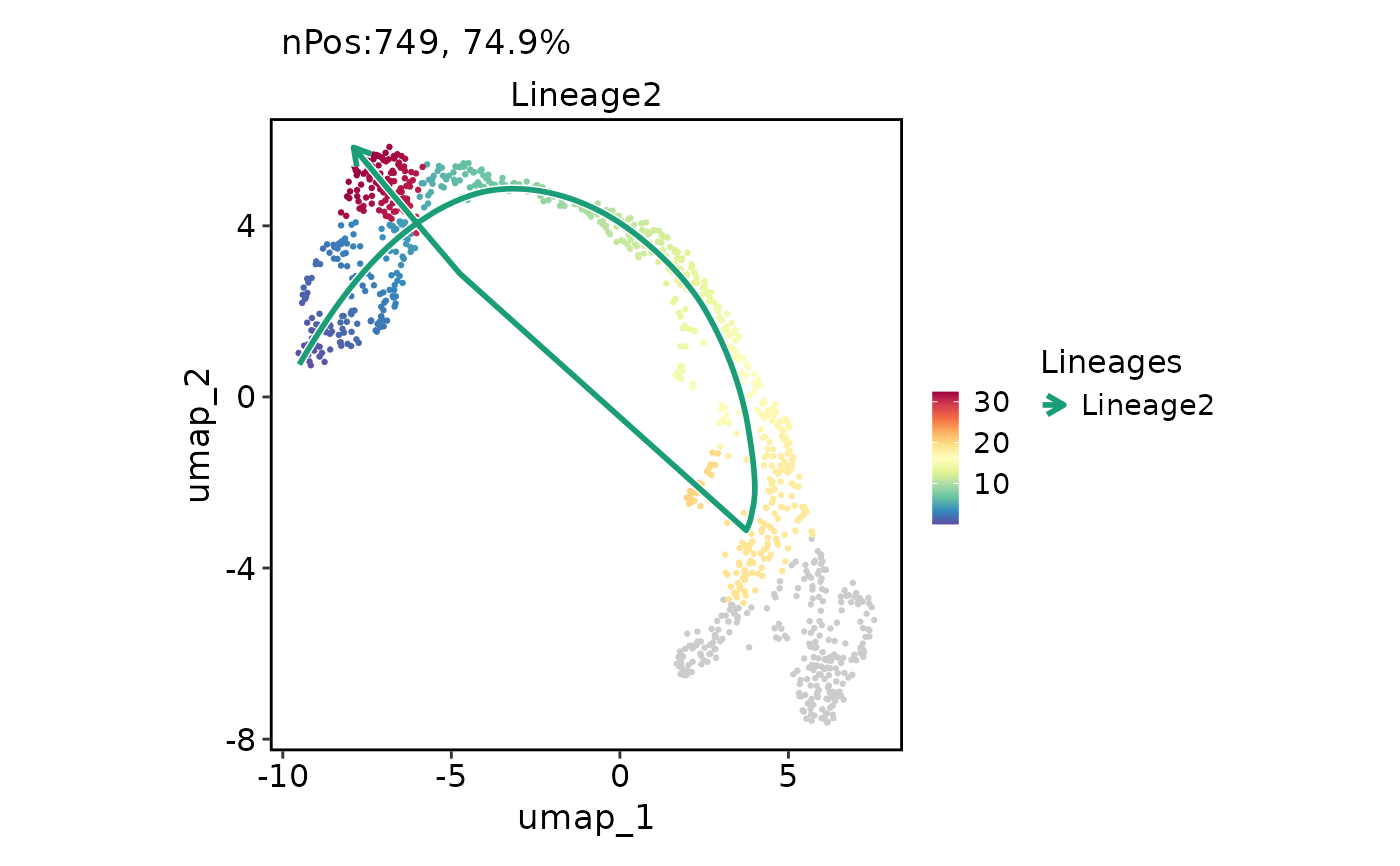
 FeatureDimPlot(
pancreas_sub,
features = "Lineage2",
reduction = "UMAP",
lineages = "Lineage2"
)
#> Warning: `guide_colourbar()` cannot be used for colour_ggnewscale_1.
#> ℹ Use one of colour, color, or fill instead.
FeatureDimPlot(
pancreas_sub,
features = "Lineage2",
reduction = "UMAP",
lineages = "Lineage2"
)
#> Warning: `guide_colourbar()` cannot be used for colour_ggnewscale_1.
#> ℹ Use one of colour, color, or fill instead.
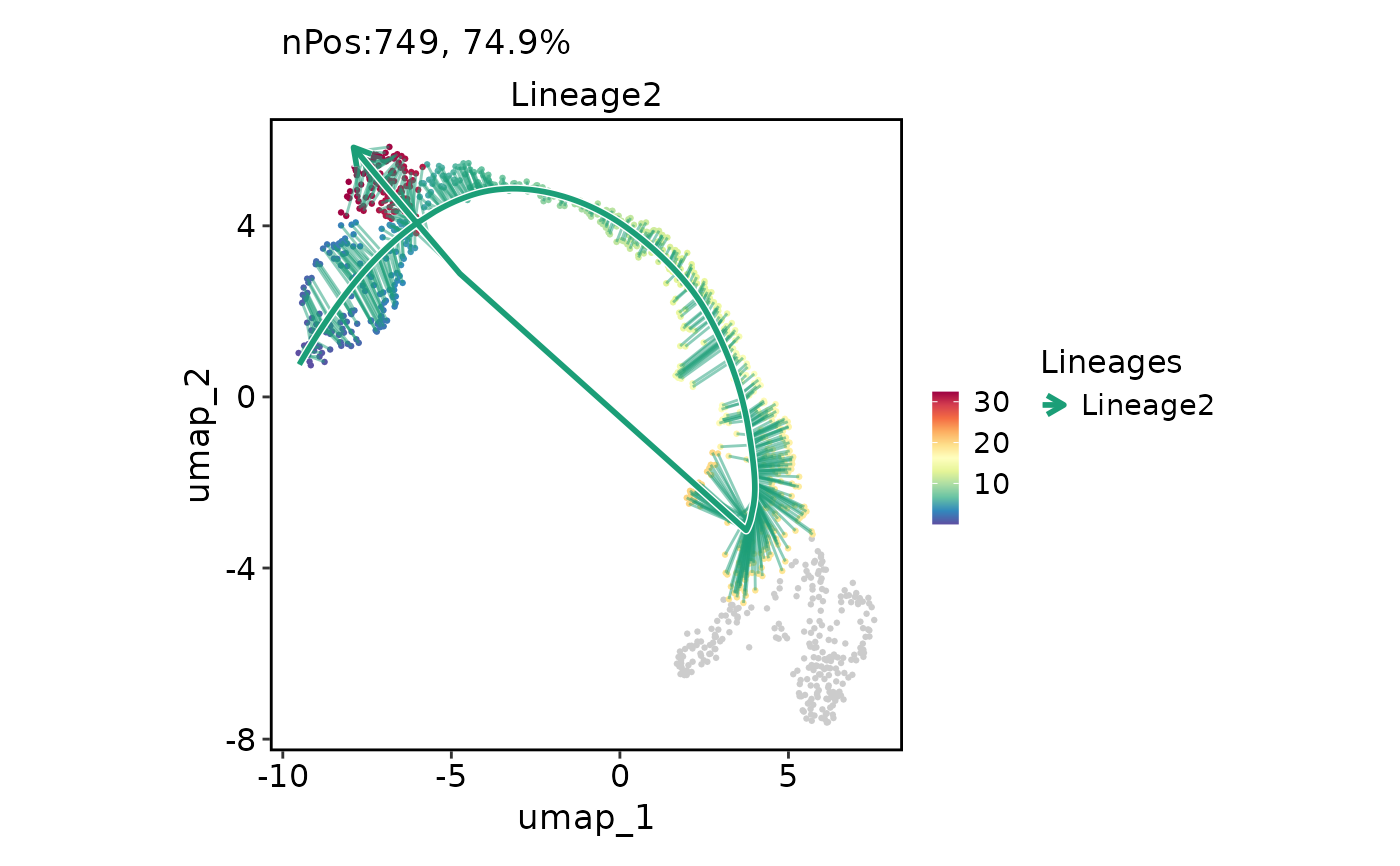
 FeatureDimPlot(
pancreas_sub,
features = "Lineage2",
reduction = "UMAP",
lineages = "Lineage2",
lineages_whiskers = TRUE
)
#> Warning: `guide_colourbar()` cannot be used for colour_ggnewscale_1.
#> ℹ Use one of colour, color, or fill instead.
FeatureDimPlot(
pancreas_sub,
features = "Lineage2",
reduction = "UMAP",
lineages = "Lineage2",
lineages_whiskers = TRUE
)
#> Warning: `guide_colourbar()` cannot be used for colour_ggnewscale_1.
#> ℹ Use one of colour, color, or fill instead.
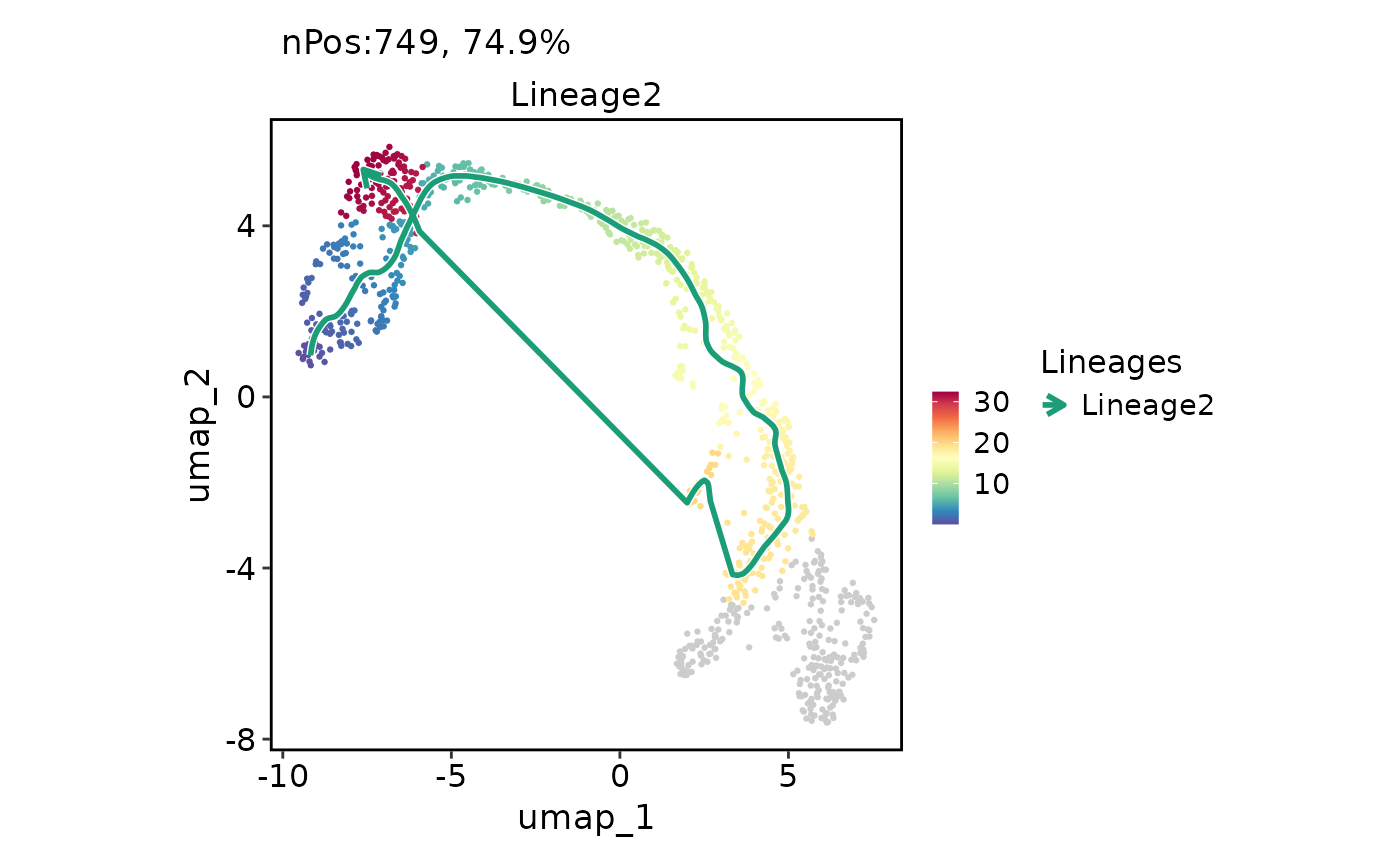
 FeatureDimPlot(
pancreas_sub,
features = "Lineage2",
reduction = "UMAP",
lineages = "Lineage2",
lineages_span = 0.1
)
#> Warning: `guide_colourbar()` cannot be used for colour_ggnewscale_1.
#> ℹ Use one of colour, color, or fill instead.
FeatureDimPlot(
pancreas_sub,
features = "Lineage2",
reduction = "UMAP",
lineages = "Lineage2",
lineages_span = 0.1
)
#> Warning: `guide_colourbar()` cannot be used for colour_ggnewscale_1.
#> ℹ Use one of colour, color, or fill instead.
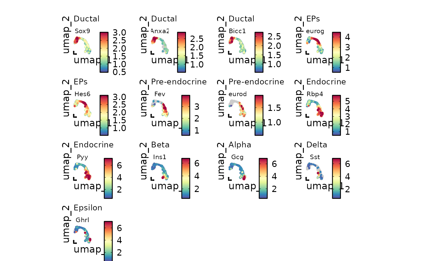
 # Input a named feature list
markers <- list(
"Ductal" = c("Sox9", "Anxa2", "Bicc1"),
"EPs" = c("Neurog3", "Hes6"),
"Pre-endocrine" = c("Fev", "Neurod1"),
"Endocrine" = c("Rbp4", "Pyy"),
"Beta" = "Ins1",
"Alpha" = "Gcg",
"Delta" = "Sst",
"Epsilon" = "Ghrl"
)
FeatureDimPlot(
pancreas_sub,
features = markers,
reduction = "UMAP",
theme_use = "theme_blank",
theme_args = list(
plot.subtitle = ggplot2::element_text(size = 10),
strip.text = ggplot2::element_text(size = 8)
)
)
# Input a named feature list
markers <- list(
"Ductal" = c("Sox9", "Anxa2", "Bicc1"),
"EPs" = c("Neurog3", "Hes6"),
"Pre-endocrine" = c("Fev", "Neurod1"),
"Endocrine" = c("Rbp4", "Pyy"),
"Beta" = "Ins1",
"Alpha" = "Gcg",
"Delta" = "Sst",
"Epsilon" = "Ghrl"
)
FeatureDimPlot(
pancreas_sub,
features = markers,
reduction = "UMAP",
theme_use = "theme_blank",
theme_args = list(
plot.subtitle = ggplot2::element_text(size = 10),
strip.text = ggplot2::element_text(size = 8)
)
)
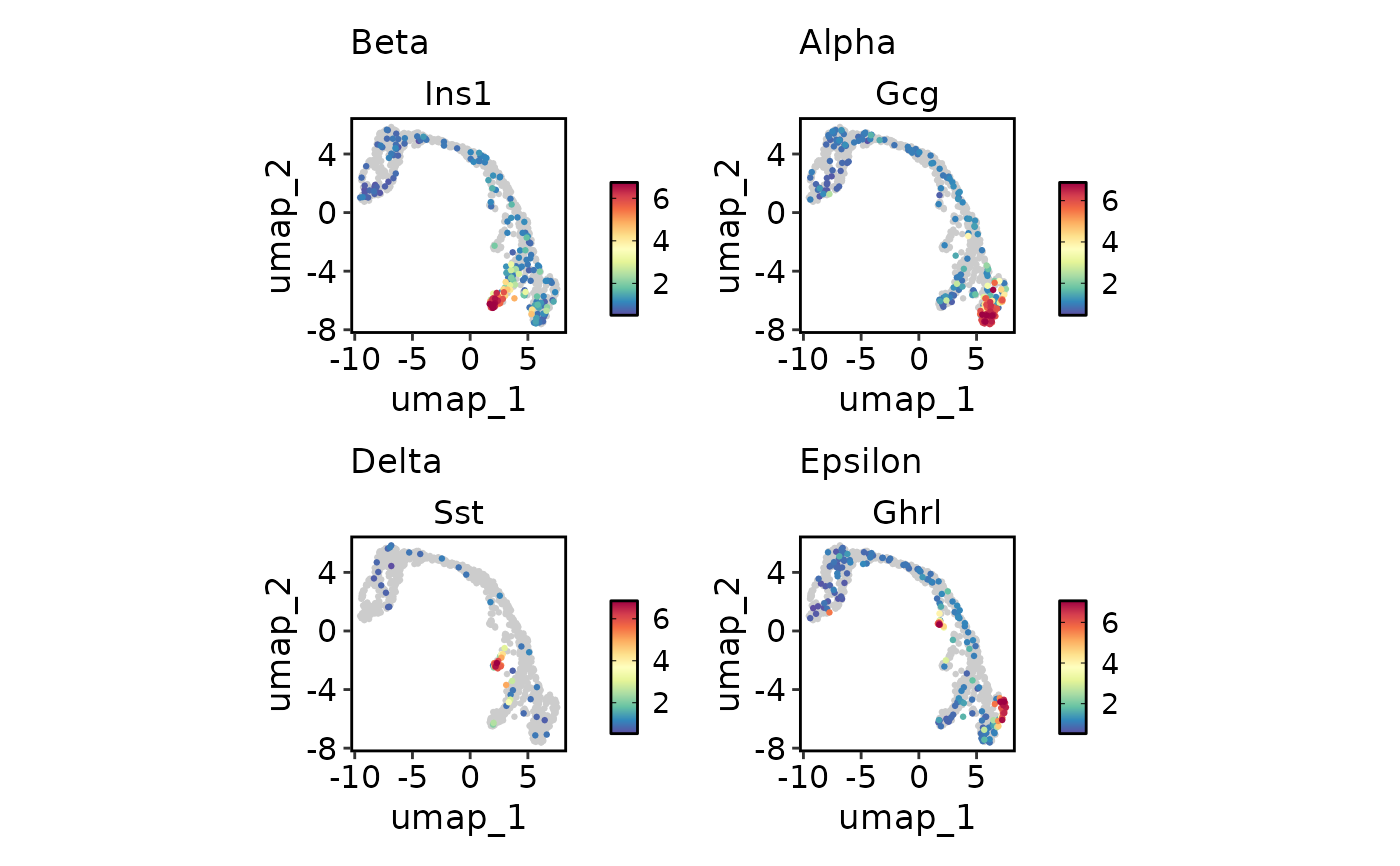
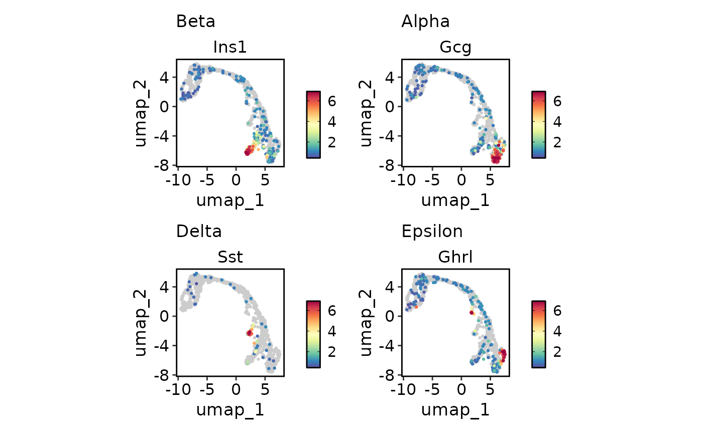
 # Plot multiple features with different scales
endocrine_markers <- c(
"Beta" = "Ins1",
"Alpha" = "Gcg",
"Delta" = "Sst",
"Epsilon" = "Ghrl"
)
FeatureDimPlot(
pancreas_sub,
endocrine_markers,
reduction = "UMAP"
)
# Plot multiple features with different scales
endocrine_markers <- c(
"Beta" = "Ins1",
"Alpha" = "Gcg",
"Delta" = "Sst",
"Epsilon" = "Ghrl"
)
FeatureDimPlot(
pancreas_sub,
endocrine_markers,
reduction = "UMAP"
)
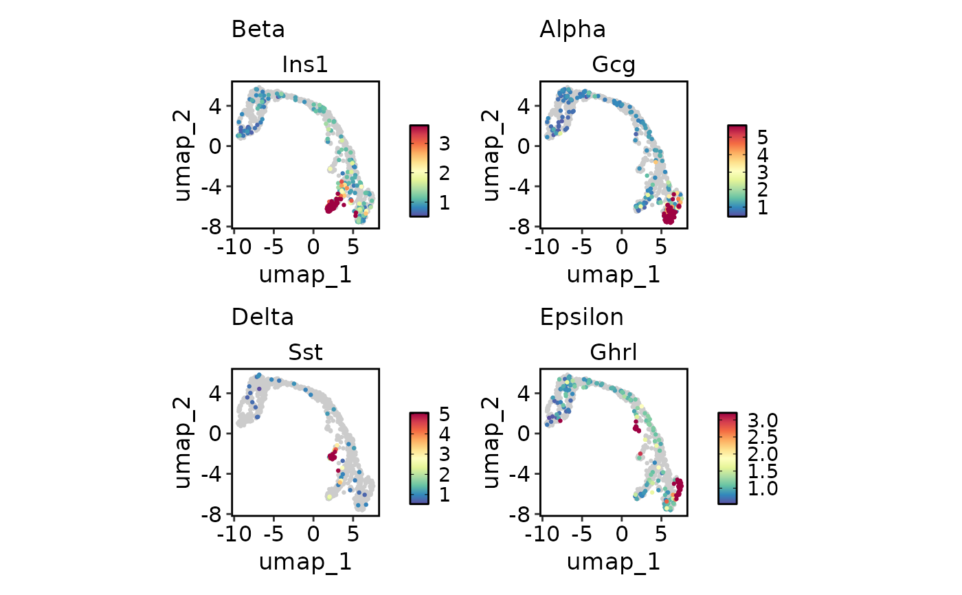
 FeatureDimPlot(
pancreas_sub,
endocrine_markers,
reduction = "UMAP",
lower_quantile = 0,
upper_quantile = 0.8
)
FeatureDimPlot(
pancreas_sub,
endocrine_markers,
reduction = "UMAP",
lower_quantile = 0,
upper_quantile = 0.8
)
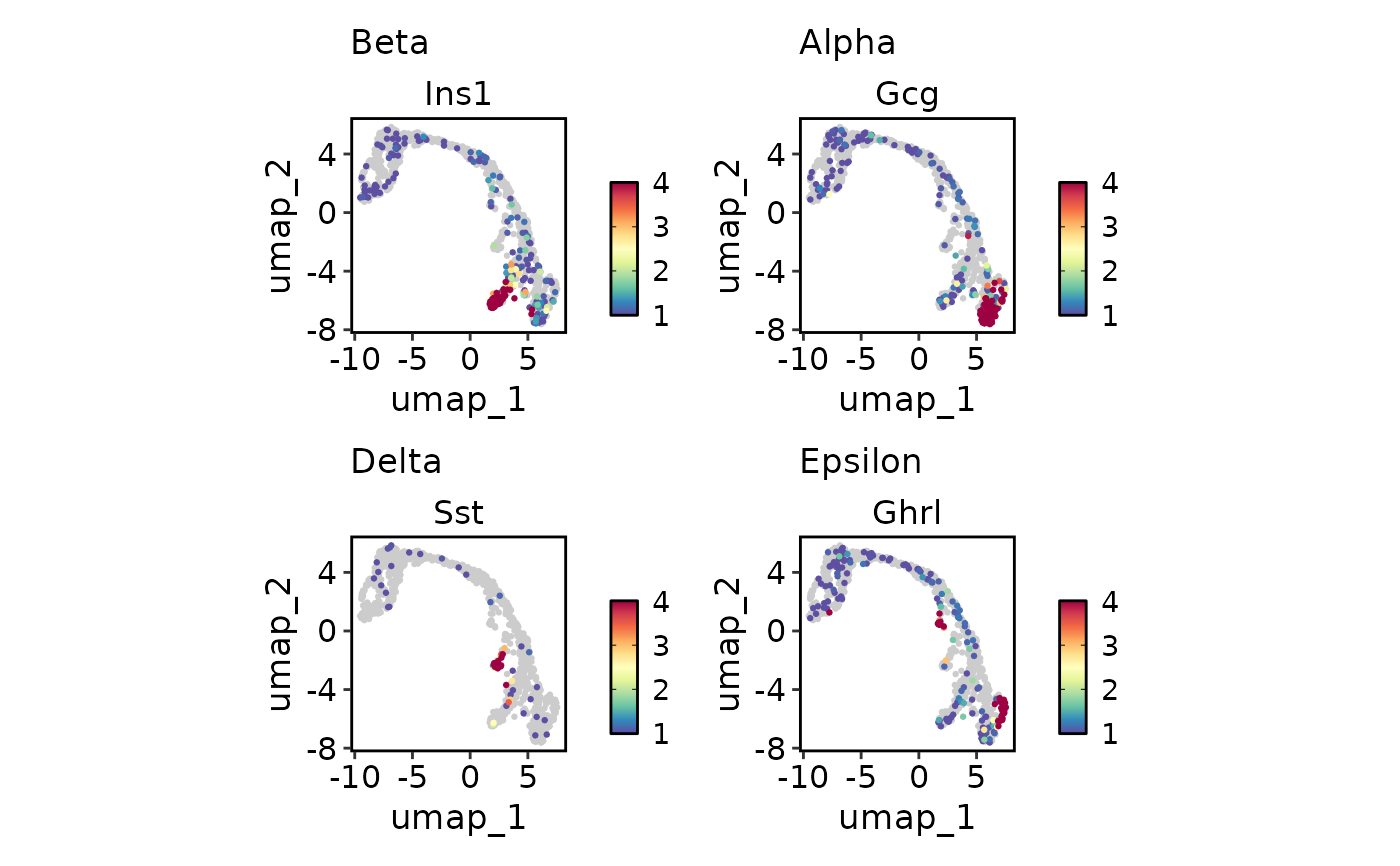
 FeatureDimPlot(
pancreas_sub,
endocrine_markers,
reduction = "UMAP",
lower_cutoff = 1,
upper_cutoff = 4
)
FeatureDimPlot(
pancreas_sub,
endocrine_markers,
reduction = "UMAP",
lower_cutoff = 1,
upper_cutoff = 4
)
 FeatureDimPlot(
pancreas_sub,
endocrine_markers,
reduction = "UMAP",
keep_scale = "all"
)
FeatureDimPlot(
pancreas_sub,
endocrine_markers,
reduction = "UMAP",
keep_scale = "all"
)
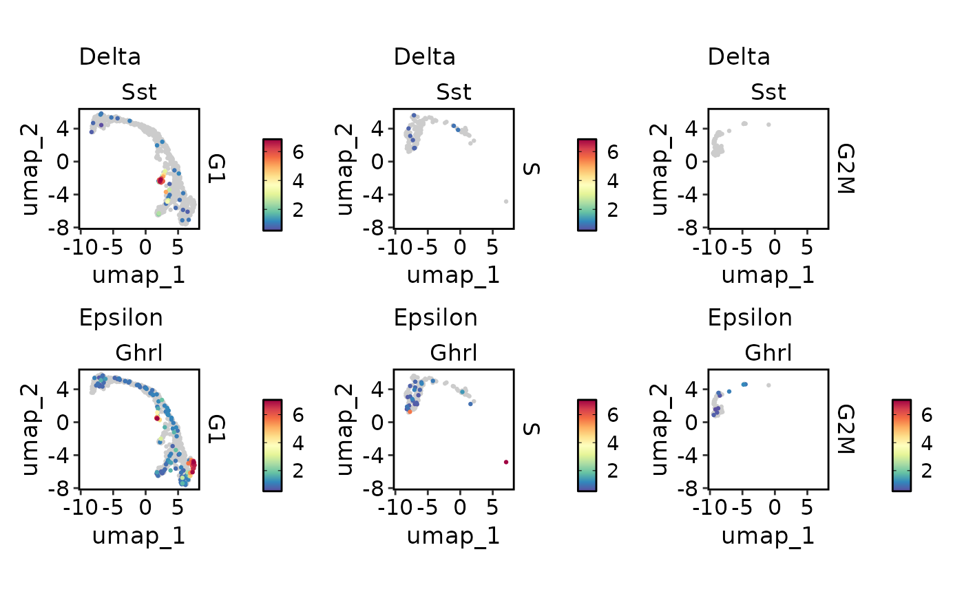
 FeatureDimPlot(
pancreas_sub,
c("Delta" = "Sst", "Epsilon" = "Ghrl"),
split.by = "Phase",
reduction = "UMAP",
keep_scale = "feature"
)
FeatureDimPlot(
pancreas_sub,
c("Delta" = "Sst", "Epsilon" = "Ghrl"),
split.by = "Phase",
reduction = "UMAP",
keep_scale = "feature"
)
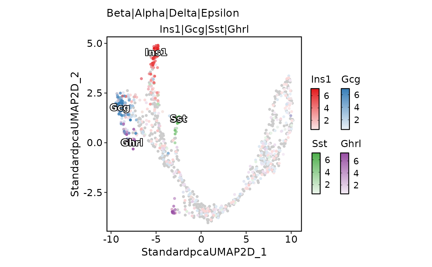
 # Plot multiple features on one picture
FeatureDimPlot(
pancreas_sub,
features = endocrine_markers,
pt.size = 1,
compare_features = TRUE,
color_blend_mode = "blend",
label = TRUE,
label_insitu = TRUE
)
#> Warning: No shared levels found between `names(values)` of the manual scale and the
#> data's colour values.
# Plot multiple features on one picture
FeatureDimPlot(
pancreas_sub,
features = endocrine_markers,
pt.size = 1,
compare_features = TRUE,
color_blend_mode = "blend",
label = TRUE,
label_insitu = TRUE
)
#> Warning: No shared levels found between `names(values)` of the manual scale and the
#> data's colour values.
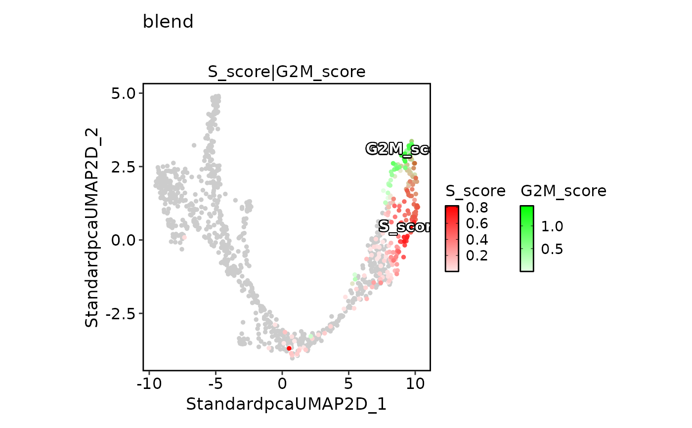
 FeatureDimPlot(
pancreas_sub,
features = c("S_score", "G2M_score"),
pt.size = 1,
palcolor = c("red", "green"),
compare_features = TRUE,
color_blend_mode = "blend",
title = "blend",
label = TRUE,
label_insitu = TRUE
)
#> Warning: No shared levels found between `names(values)` of the manual scale and the
#> data's colour values.
FeatureDimPlot(
pancreas_sub,
features = c("S_score", "G2M_score"),
pt.size = 1,
palcolor = c("red", "green"),
compare_features = TRUE,
color_blend_mode = "blend",
title = "blend",
label = TRUE,
label_insitu = TRUE
)
#> Warning: No shared levels found between `names(values)` of the manual scale and the
#> data's colour values.
 FeatureDimPlot(
pancreas_sub,
features = c("S_score", "G2M_score"),
pt.size = 1,
palcolor = c("red", "green"),
compare_features = TRUE,
color_blend_mode = "average",
title = "average",
label = TRUE,
label_insitu = TRUE
)
#> Warning: No shared levels found between `names(values)` of the manual scale and the
#> data's colour values.
FeatureDimPlot(
pancreas_sub,
features = c("S_score", "G2M_score"),
pt.size = 1,
palcolor = c("red", "green"),
compare_features = TRUE,
color_blend_mode = "average",
title = "average",
label = TRUE,
label_insitu = TRUE
)
#> Warning: No shared levels found between `names(values)` of the manual scale and the
#> data's colour values.
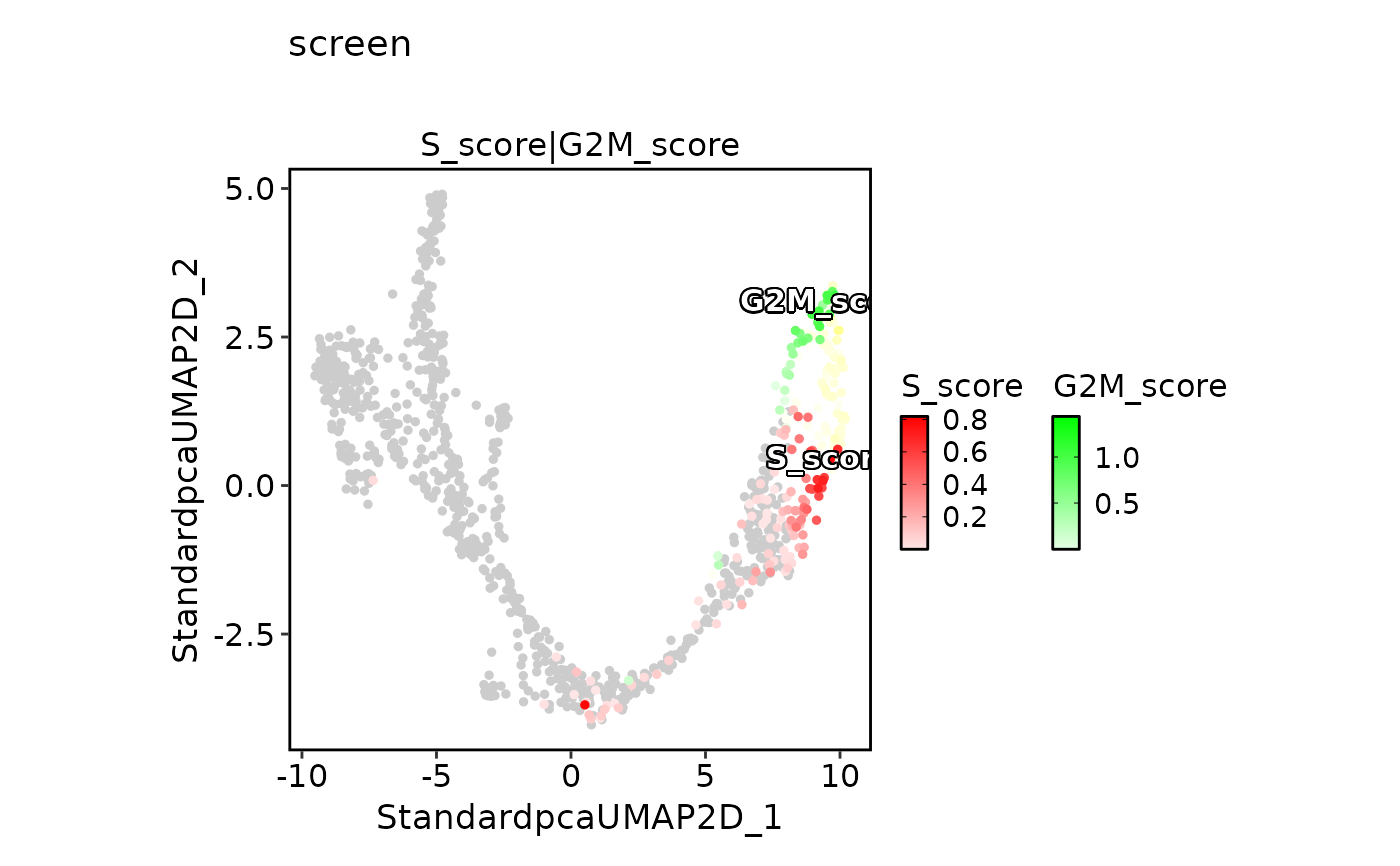
 FeatureDimPlot(
pancreas_sub,
features = c("S_score", "G2M_score"),
pt.size = 1,
palcolor = c("red", "green"),
compare_features = TRUE,
color_blend_mode = "screen",
title = "screen",
label = TRUE,
label_insitu = TRUE
)
#> Warning: No shared levels found between `names(values)` of the manual scale and the
#> data's colour values.
FeatureDimPlot(
pancreas_sub,
features = c("S_score", "G2M_score"),
pt.size = 1,
palcolor = c("red", "green"),
compare_features = TRUE,
color_blend_mode = "screen",
title = "screen",
label = TRUE,
label_insitu = TRUE
)
#> Warning: No shared levels found between `names(values)` of the manual scale and the
#> data's colour values.
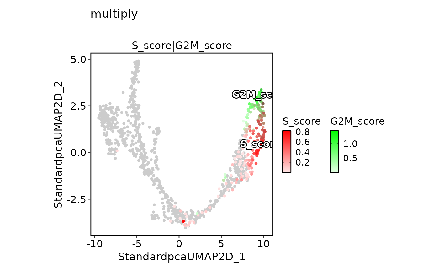
 FeatureDimPlot(
pancreas_sub,
features = c("S_score", "G2M_score"),
pt.size = 1,
palcolor = c("red", "green"),
compare_features = TRUE,
color_blend_mode = "multiply",
title = "multiply",
label = TRUE,
label_insitu = TRUE
)
#> Warning: No shared levels found between `names(values)` of the manual scale and the
#> data's colour values.
FeatureDimPlot(
pancreas_sub,
features = c("S_score", "G2M_score"),
pt.size = 1,
palcolor = c("red", "green"),
compare_features = TRUE,
color_blend_mode = "multiply",
title = "multiply",
label = TRUE,
label_insitu = TRUE
)
#> Warning: No shared levels found between `names(values)` of the manual scale and the
#> data's colour values.