Introduction
The scop package provides a unified and extensible framework for single-cell omics data processing and downstream analysis in Seurat:
- Integrated single-cell quality control methods, including doublet detection methods (scDblFinder, scds, Scrublet, DoubletDetection) and ambient RNA decontamination via decontX.
- Pipelines embedded with multiple methods for normalization, feature reduction (PCA, ICA, NMF, MDS, GLMPCA, UMAP, TriMap, LargeVis, PaCMAP, PHATE, DM, FR), and cell population identification.
- Pipelines embedded with multiple integration methods for scRNA-seq, including Uncorrected, Seurat, scVI, MNN, fastMNN, Harmony, Scanorama, BBKNN, CSS, LIGER, Conos, ComBat.
- Multiple methods for automatic annotation of single-cell data (CellTypist, SingleR, Scmap, KNNPredict) and methods for projection between single-cell datasets (CSSMap, PCAMap, SeuratMap, SymphonyMap).
- Multiple single-cell downstream analyses:
- Differential expression analysis: identification of differential features, expressed marker identification.
- Enrichment analysis: over-representation analysis, GSEA analysis, dynamic enrichment analysis.
- Cellular potency: CytoTRACE 2 for predicting cellular differentiation potential.
- RNA velocity: RNA velocity, PAGA, Palantir, CellRank, WOT.
- Trajectory inference: Slingshot, Monocle2, Monocle3, identification of dynamic features.
- Cell-Cell Communication: CellChat for cell-cell communication.
- High-quality data visualization methods.
- Fast deployment of single-cell data into SCExplorer, a shiny app that provides an interactive visualization interface.
Table of Contents
-
scop: Single-Cell Omics analysis Pipeline
- Introduction
- Table of Contents
- Credits
- Installation
- Pipeline
Credits
The scop package is developed based on the SCP package, with the following major improvements:
- Compatibility: full support for Seurat v5.
- Stability: a large number of known issues have been fixed, and all functions have passed
devtools::check(). - Usability: the Python environment setup workflow has been improved, allowing a new complete environment to be deployed within minutes; standardized console messages via
thisutils::log_messagefor consistent, readable function outputs. - Performance: a new parallel framework has been developed based on
thisutils::parallelize_fun, providing a consistent experience across Linux, macOS, and Windows. - Functionality: more analysis methods have been added, including CellRank, CellTypist, CytoTRACE 2, CellChat, GSVA, scMetabolism and scProportionTest.
Installation
R requirement
- R >= 4.1.0
You can install the latest version of scop with pak from GitHub with:
if (!require("pak", quietly = TRUE)) {
  install.packages("pak")
}
pak::pak("mengxu98/scop")
Python environment
To run functions such as RunPAGA(), RunSCVELO(), scop requires conda to create a separate environment. The default environment name is "scop_env". You can specify the environment name for scop by setting options(scop_envname = "new_name").
Now, you can run PrepareEnv() to create the python environment for scop. If the conda binary is not found, it will automatically download and install miniconda.
scop::PrepareEnv()To force scop to use a specific conda binary, it is recommended to set reticulate.conda_binary R option:
options(reticulate.conda_binary = "/path/to/conda")
scop::PrepareEnv()
If the download of miniconda or pip packages is slow, you can specify the miniconda repo and PyPI mirror according to your network region.
scop::PrepareEnv(
  miniconda_repo = "https://mirrors.bfsu.edu.cn/anaconda/miniconda",
  pip_options = "-i https://pypi.tuna.tsinghua.edu.cn/simple"
)- Available miniconda repositories:
- https://repo.anaconda.com/miniconda (default)
- http://mirrors.aliyun.com/anaconda/miniconda
- https://mirrors.bfsu.edu.cn/anaconda/miniconda
- https://mirrors.pku.edu.cn/anaconda/miniconda
- https://mirror.nju.edu.cn/anaconda/miniconda
- https://mirrors.sustech.edu.cn/anaconda/miniconda
- https://mirrors.xjtu.edu.cn/anaconda/miniconda
- https://mirrors.hit.edu.cn/anaconda/miniconda
- Available PyPI mirrors:
- https://pypi.python.org/simple (default)
- https://mirrors.aliyun.com/pypi/simple
- https://pypi.tuna.tsinghua.edu.cn/simple
- https://mirrors.pku.edu.cn/pypi/simple
- https://mirror.nju.edu.cn/pypi/web/simple
- https://mirrors.sustech.edu.cn/pypi/simple
- https://mirrors.xjtu.edu.cn/pypi/simple
- https://mirrors.hit.edu.cn/pypi/web/simple
Pipeline
Data exploration
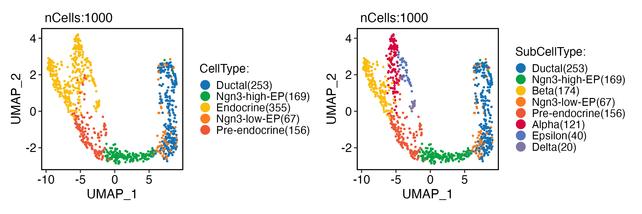
The analysis is based on a subsetted version of mouse pancreas data.
library(scop)
data(pancreas_sub)
print(pancreas_sub)
#> An object of class Seurat
#> 47994 features across 1000 samples within 3 assays
#> Active assay: RNA (15998 features, 0 variable features)
#>  1 layer present: counts
#>  2 other assays present: spliced, unspliced
pancreas_sub <- standard_scop(pancreas_sub)
print(pancreas_sub)
#>  An object of class Seurat
#>  47994 features across 1000 samples within 3 assays
#>  Active assay: RNA (15998 features, 2000 variable features)
#>   3 layers present: counts, data, scale.data
#>   2 other assays present: spliced, unspliced
#>   5 dimensional reductions calculated: Standardpca, StandardpcaUMAP2D, StandardpcaUMAP3D, StandardUMAP2D, StandardUMAP3D
CellDimPlot(
  pancreas_sub,
  group.by = c("CellType", "SubCellType"),
  reduction = "UMAP",
  xlab = "UMAP_1",
  ylab = "UMAP_2"
)
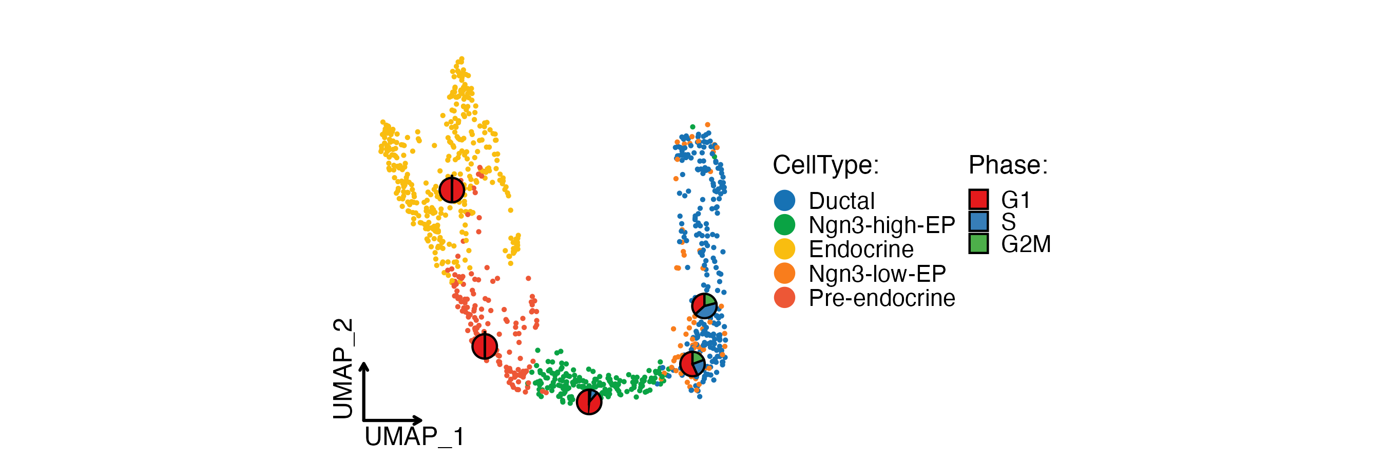
CellDimPlot(
  pancreas_sub,
  group.by = "SubCellType",
  stat.by = "Phase",
  reduction = "UMAP",
  theme_use = "theme_blank",
  xlab = "UMAP_1",
  ylab = "UMAP_2"
)
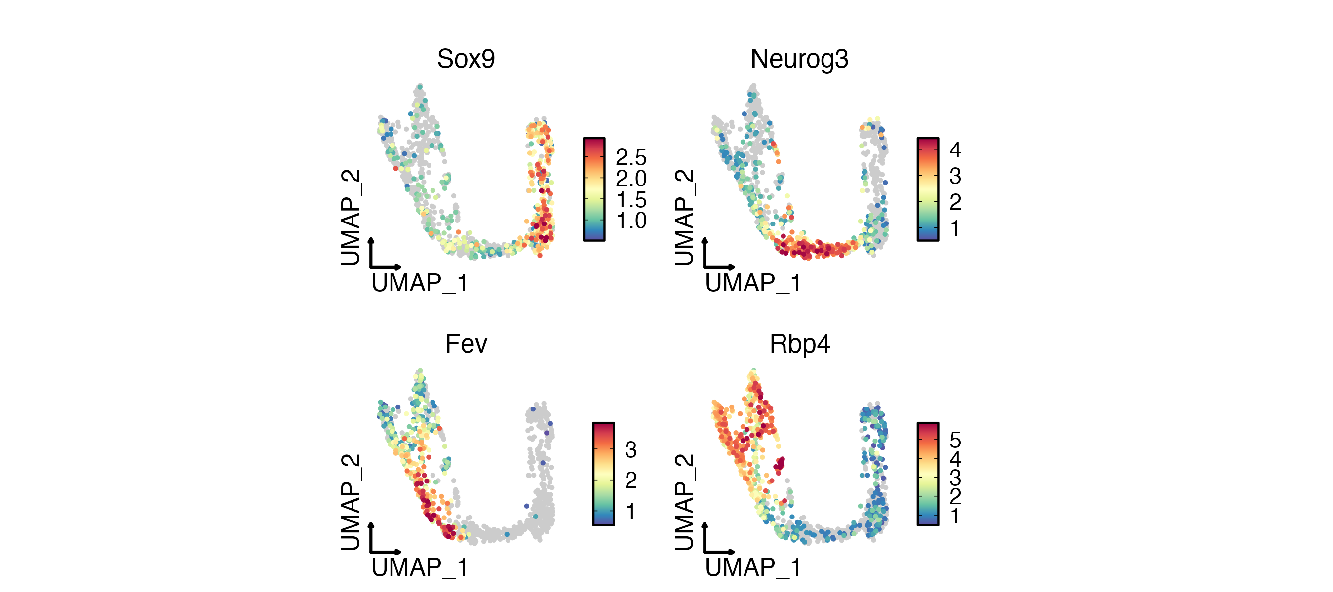
FeatureDimPlot(
  pancreas_sub,
  features = c("Sox9", "Neurog3", "Fev", "Rbp4"),
  reduction = "UMAP",
  theme_use = "theme_blank",
  xlab = "UMAP_1",
  ylab = "UMAP_2"
)
FeatureDimPlot(
  pancreas_sub,
  features = c("Ins1", "Gcg", "Sst", "Ghrl"),
  compare_features = TRUE,
  label = TRUE,
  label_insitu = TRUE,
  reduction = "UMAP",
  theme_use = "theme_blank",
  xlab = "UMAP_1",
  ylab = "UMAP_2"
)
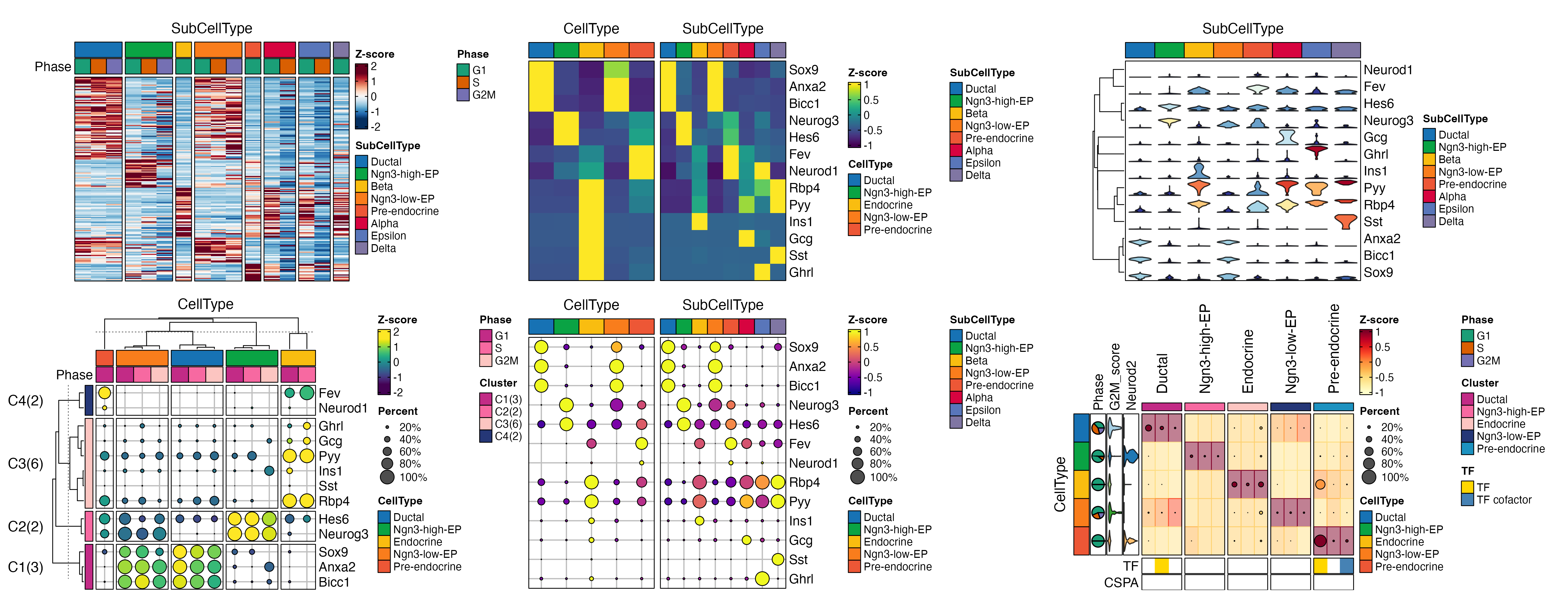
ht <- GroupHeatmap(
  pancreas_sub,
  features = c(
    "Sox9", "Anxa2", # Ductal
    "Neurog3", "Hes6", # EPs
    "Fev", "Neurod1", # Pre-endocrine
    "Rbp4", "Pyy", # Endocrine
    "Ins1", "Gcg", "Sst", "Ghrl" # Beta, Alpha, Delta, Epsilon
  ),
  group.by = c("CellType", "SubCellType"),
  heatmap_palette = "Spectral",
  cell_annotation = c("Phase", "G2M_score", "Cdh2"),
  cell_annotation_palette = c("Dark2", "Chinese", "Chinese"),
  show_row_names = TRUE,
  nlabel = 0,
  row_names_side = "left",
  add_dot = TRUE,
  add_reticle = TRUE,
  width = 2.2,
  height = 2.5
)
print(ht$plot)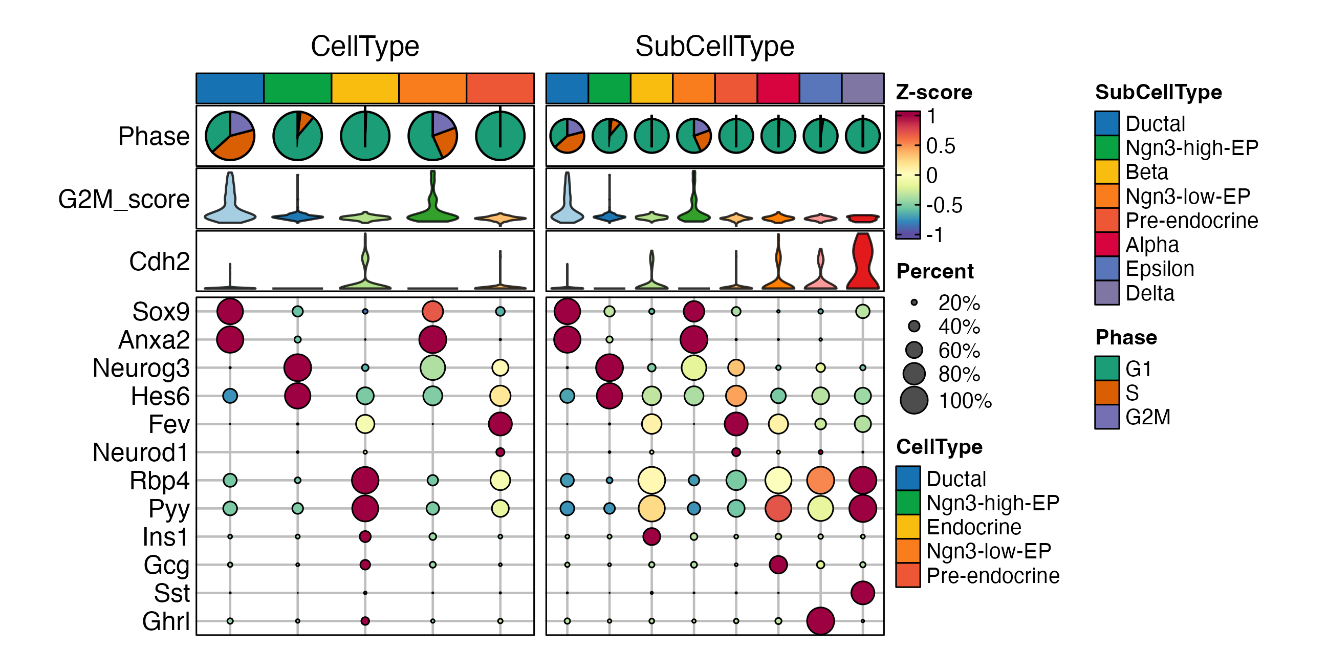
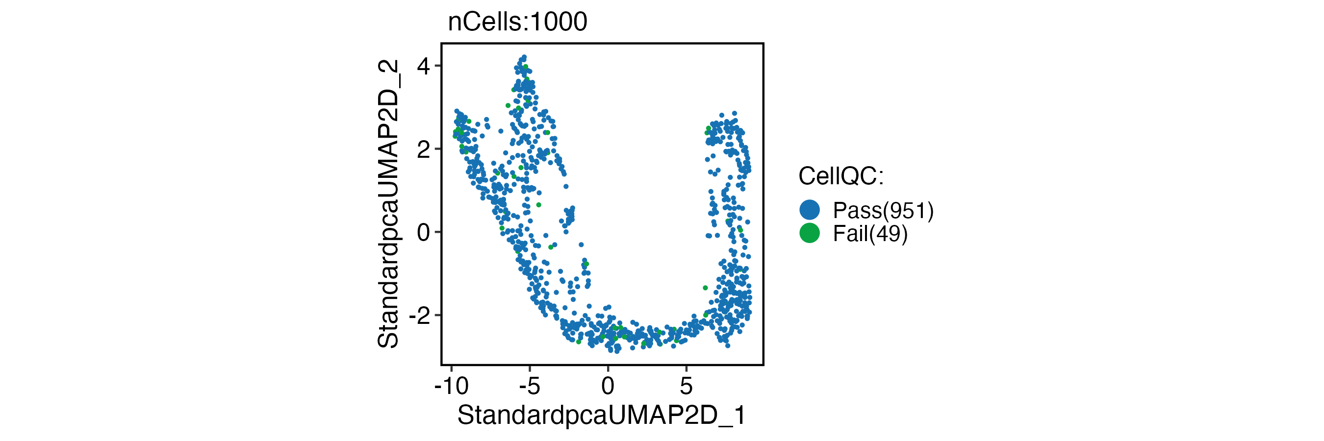
Quality control
pancreas_sub <- RunCellQC(pancreas_sub)
CellDimPlot(
  pancreas_sub,
  group.by = "CellQC",
  reduction = "UMAP"
)
CellStatPlot(
  pancreas_sub,
  stat.by = "CellQC",
  group.by = "CellType"
) + ggplot2::theme(aspect.ratio = 1 / 2)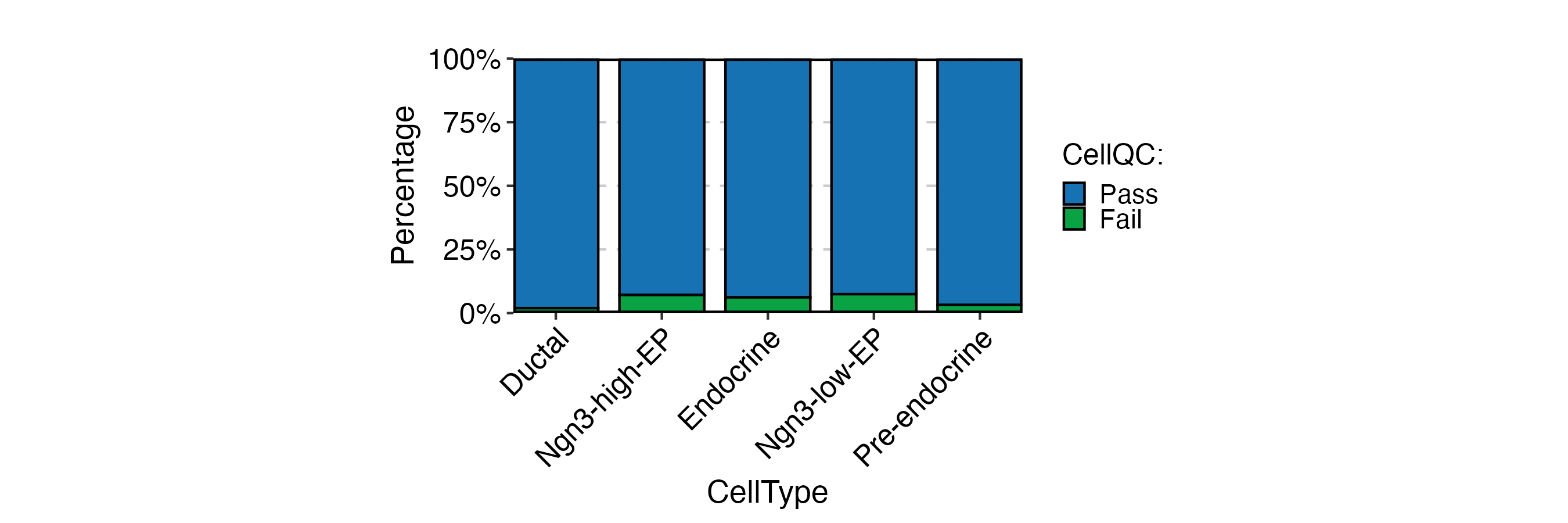
CellStatPlot(
  pancreas_sub,
  stat.by = c(
    "db_qc", "decontX_qc", "outlier_qc",
    "umi_qc", "gene_qc",
    "mito_qc", "ribo_qc",
    "ribo_mito_ratio_qc", "species_qc"
  ),
  plot_type = "upset",
  stat_level = "Fail"
) + ggplot2::theme(aspect.ratio = 1 / 2)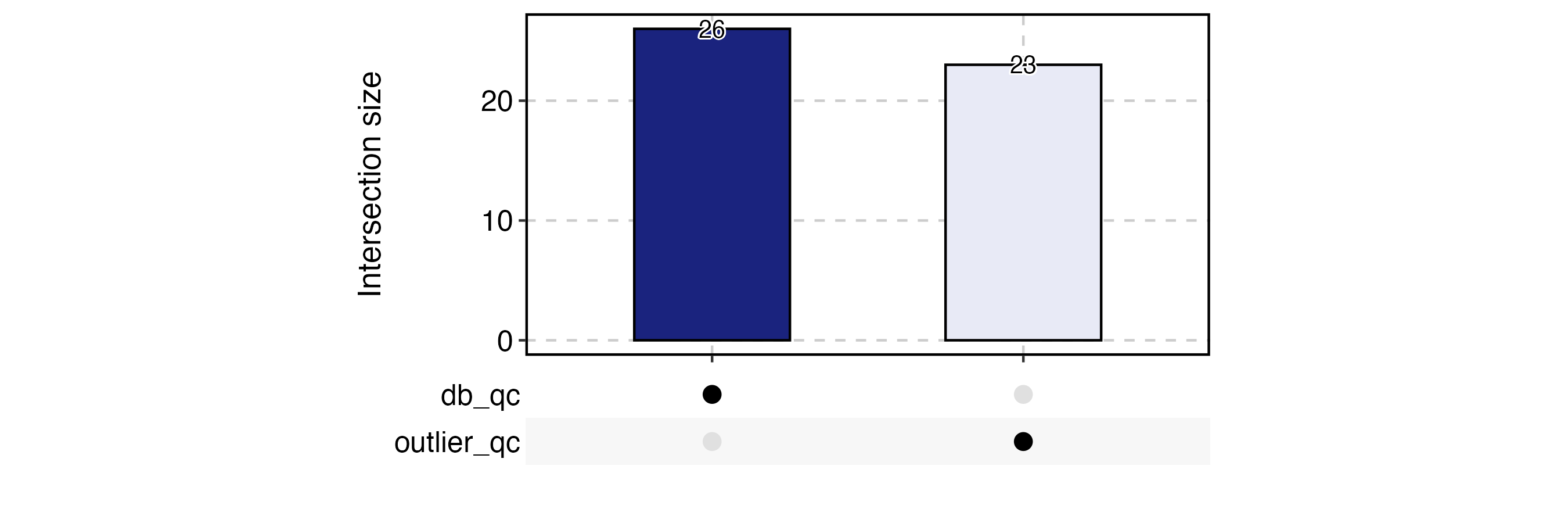
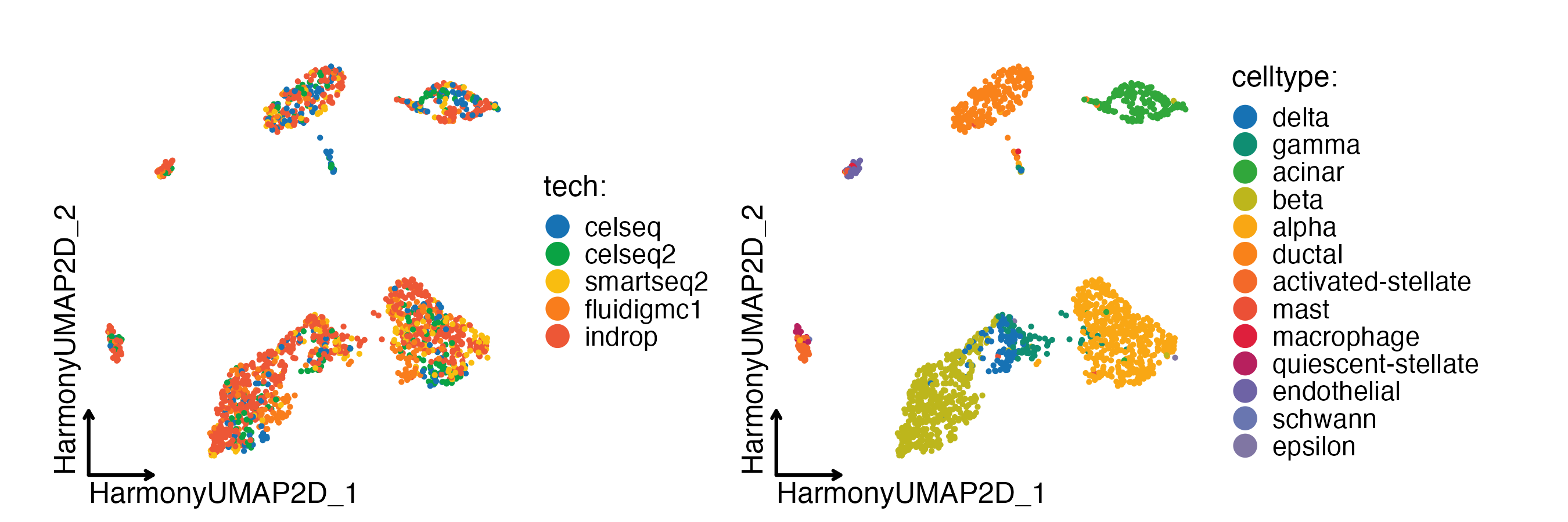
Integration pipeline
Example data for integration is a subsetted version of panc8(eight human pancreas datasets)
data(panc8_sub)
panc8_sub <- integration_scop(
  srt_merge = panc8_sub,
  batch = "tech",
  integration_method = "Harmony"
)
CellDimPlot(
  panc8_sub,
  group.by = c("tech", "celltype"),
  reduction = "HarmonyUMAP",
  theme_use = "theme_blank"
)
Cell annotation
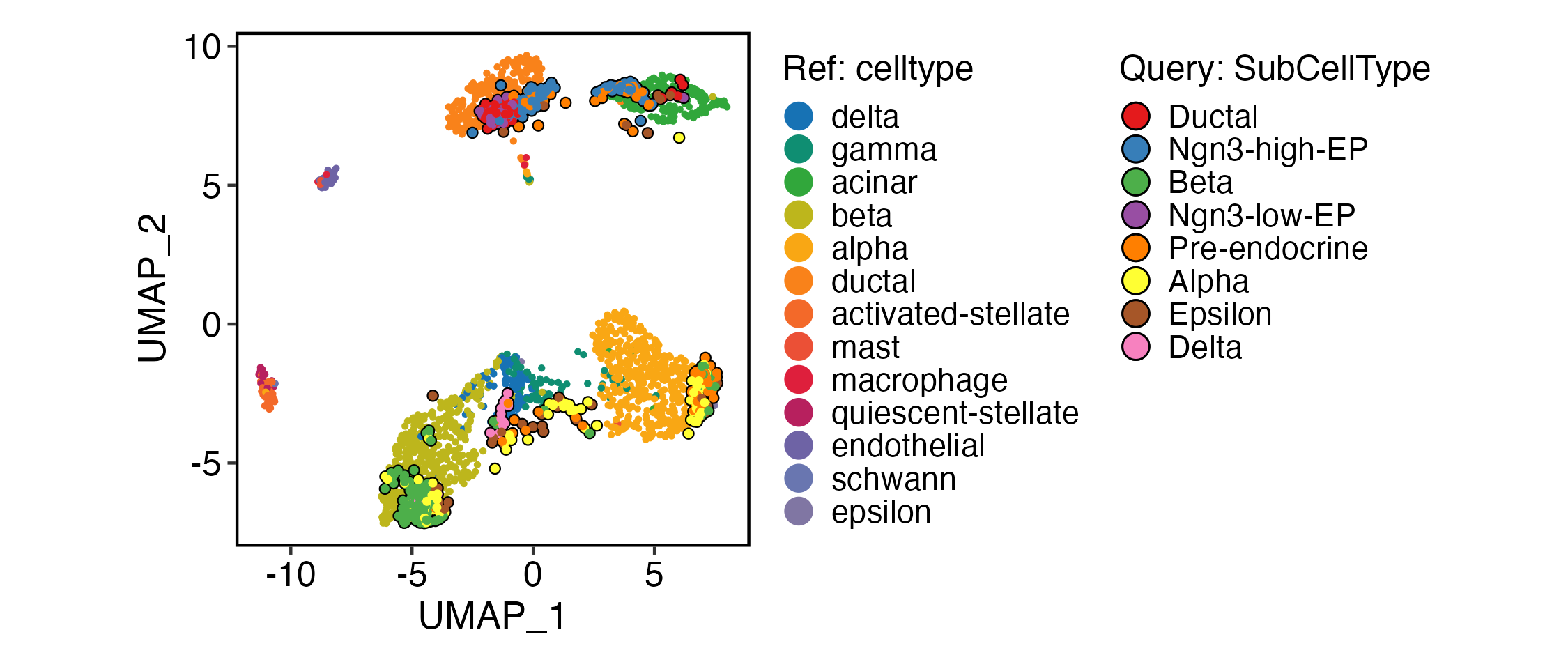
Cell projection between single-cell datasets
genenames <- make.unique(
  thisutils::capitalize(
    rownames(panc8_sub[["RNA"]]),
    force_tolower = TRUE
  )
)
names(genenames) <- rownames(panc8_sub)
panc8_rename <- RenameFeatures(
  panc8_sub,
  newnames = genenames,
  assays = "RNA"
)
srt_query <- RunKNNMap(
  srt_query = pancreas_sub,
  srt_ref = panc8_rename,
  ref_umap = "HarmonyUMAP2D"
)
ProjectionPlot(
  srt_query = srt_query,
  srt_ref = panc8_rename,
  query_group = "SubCellType",
  ref_group = "celltype",
  ref_param = list(
    xlab = "UMAP_1",
    ylab = "UMAP_2"
  )
)
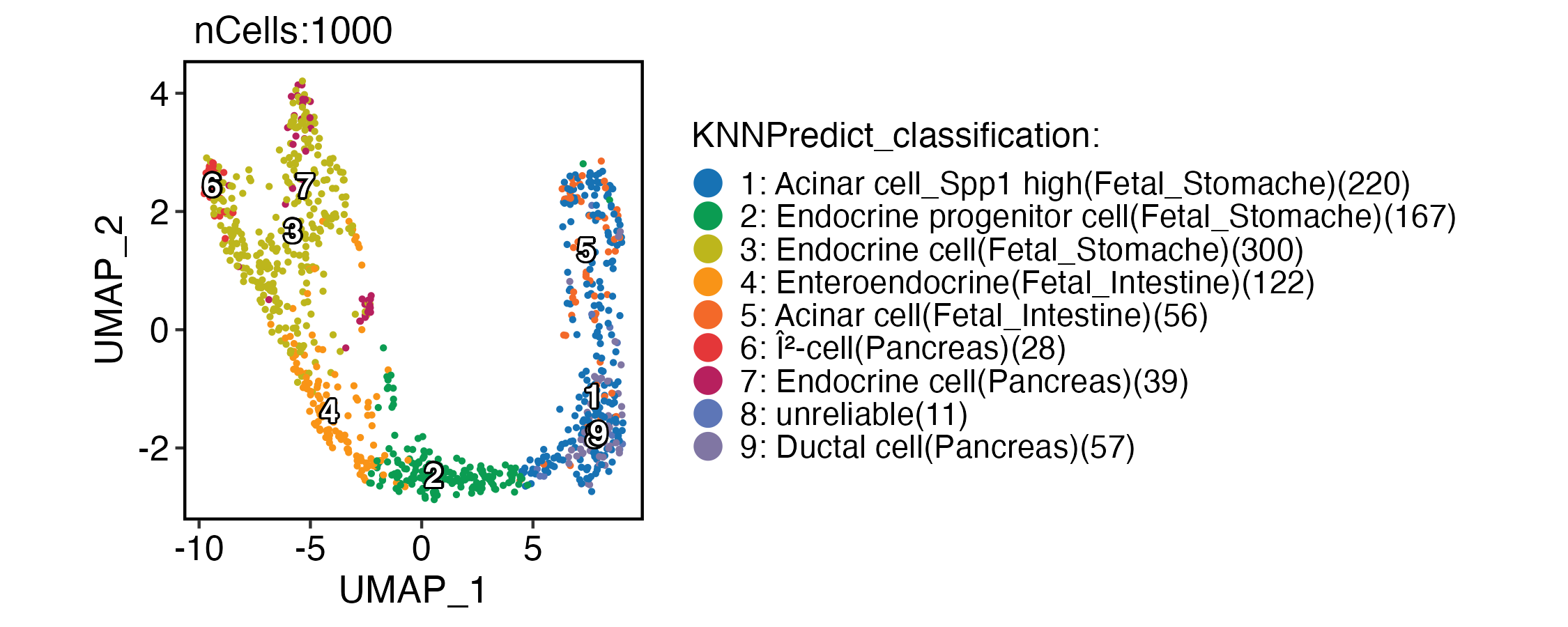
Cell annotation using bulk RNA-seq datasets
data(ref_scMCA)
pancreas_sub <- RunKNNPredict(
  srt_query = pancreas_sub,
  bulk_ref = ref_scMCA,
  filter_lowfreq = 20
)
CellDimPlot(
  pancreas_sub,
  group.by = "KNNPredict_classification",
  reduction = "UMAP",
  label = TRUE,
  xlab = "UMAP_1",
  ylab = "UMAP_2"
)
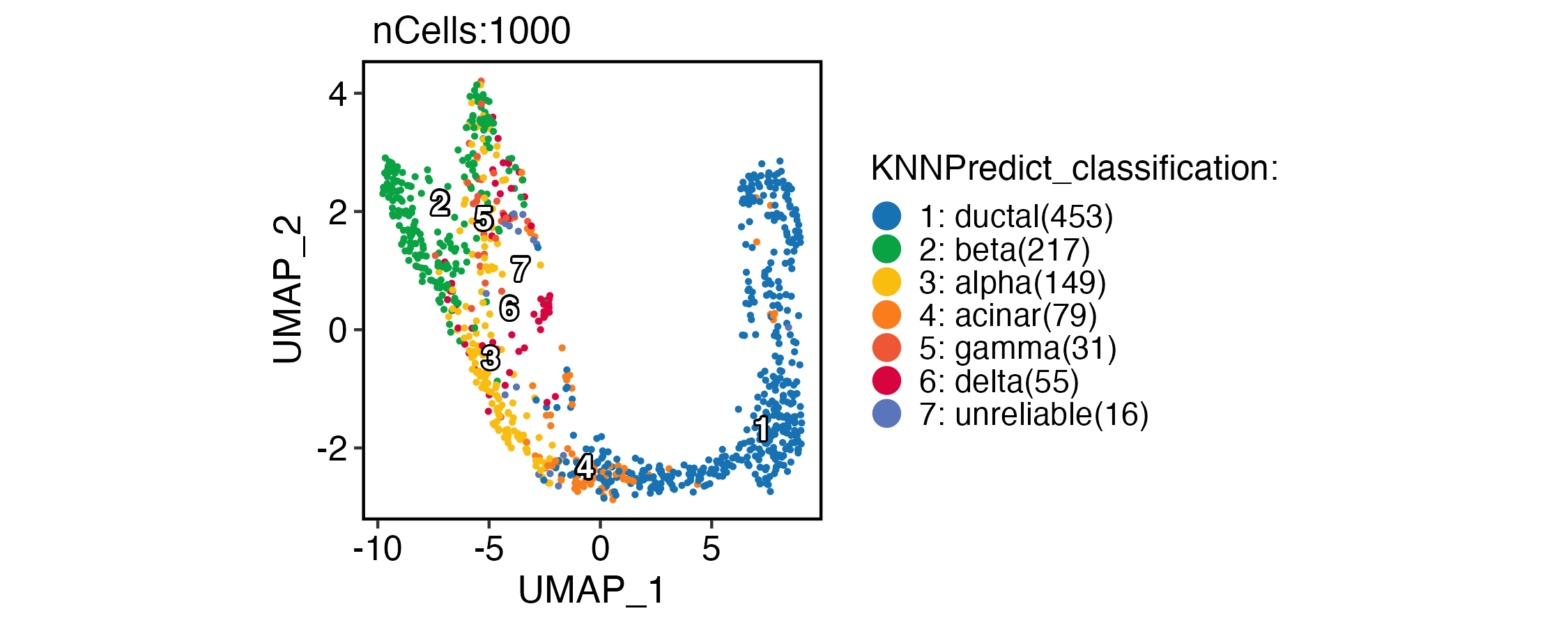
Cell annotation using single-cell datasets
pancreas_sub <- RunKNNPredict(
  srt_query = pancreas_sub,
  srt_ref = panc8_rename,
  ref_group = "celltype",
  filter_lowfreq = 20
)
CellDimPlot(
  pancreas_sub,
  group.by = "KNNPredict_classification",
  reduction = "UMAP",
  label = TRUE,
  xlab = "UMAP_1",
  ylab = "UMAP_2"
)
ht <- CellCorHeatmap(
  srt_query = pancreas_sub,
  srt_ref = panc8_rename,
  query_group = "SubCellType",
  ref_group = "celltype",
  nlabel = 3,
  label_by = "row",
  show_row_names = TRUE,
  show_column_names = TRUE,
  width = 4,
  height = 2.5
)
print(ht$plot)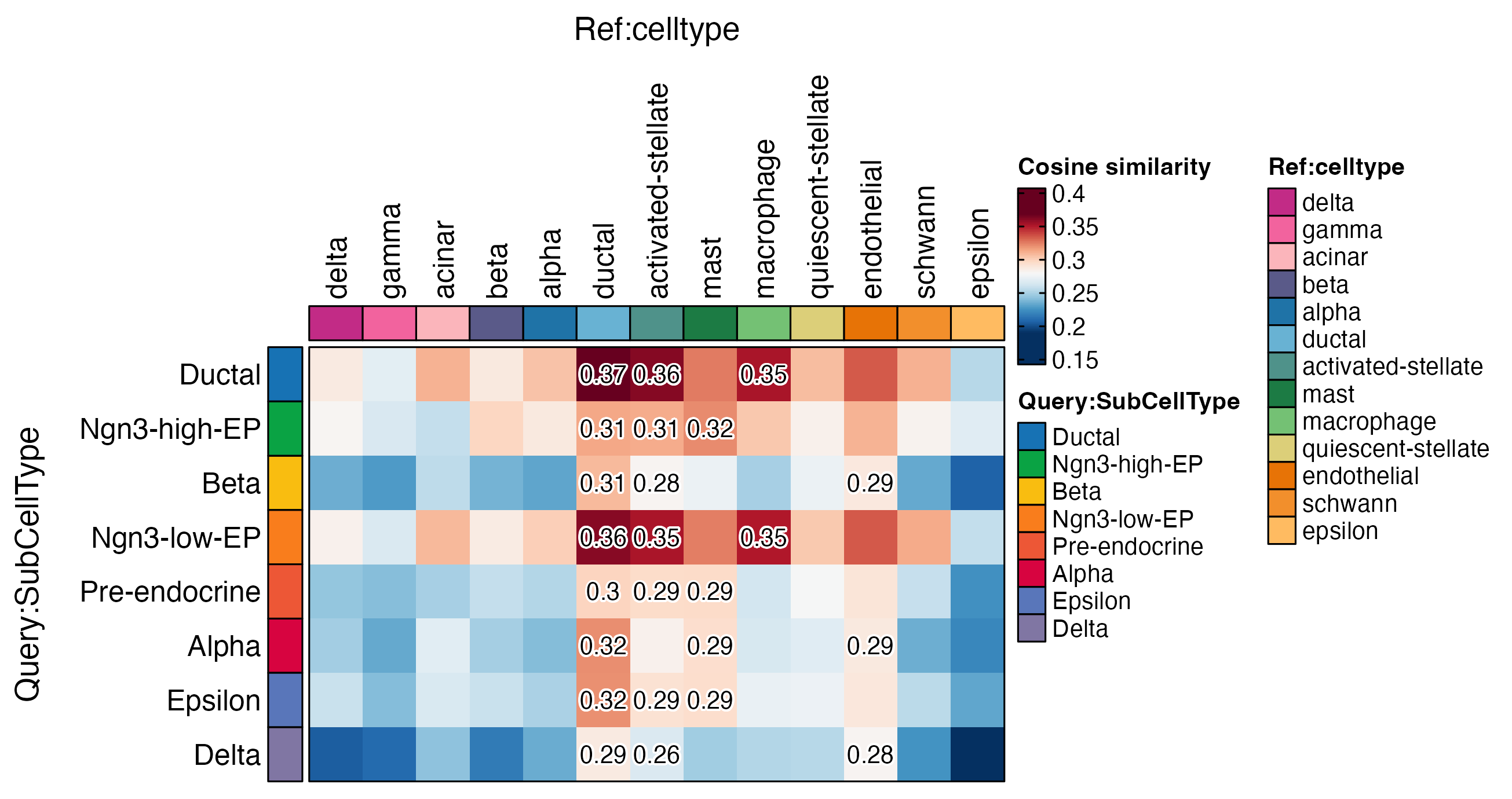
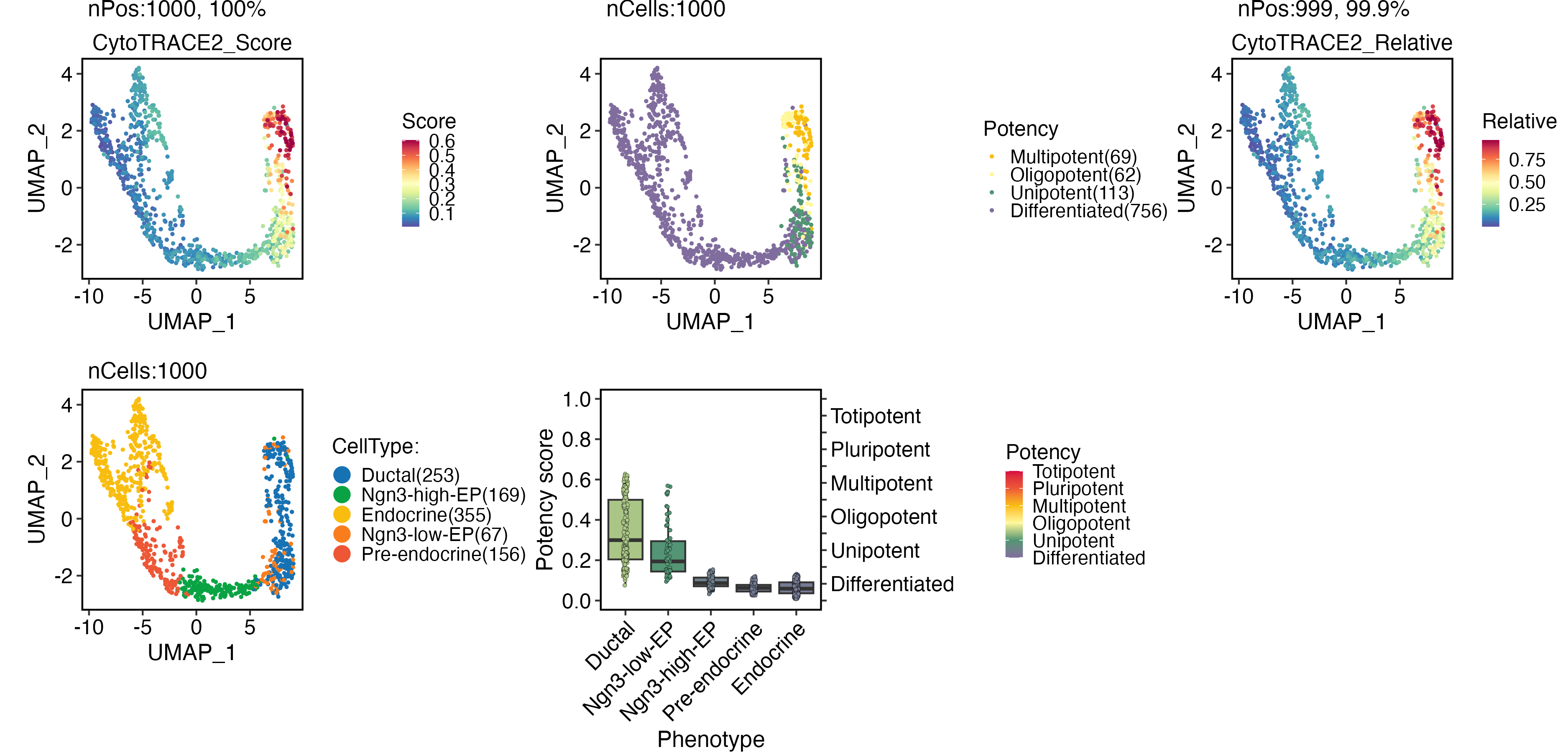
Cellular potency
CytoTRACE 2
pancreas_sub <- RunCytoTRACE(
  pancreas_sub,
  species = "Mus_musculus"
)
CytoTRACEPlot(
  pancreas_sub,
  group.by = "CellType",
  xlab = "UMAP_1",
  ylab = "UMAP_2"
)
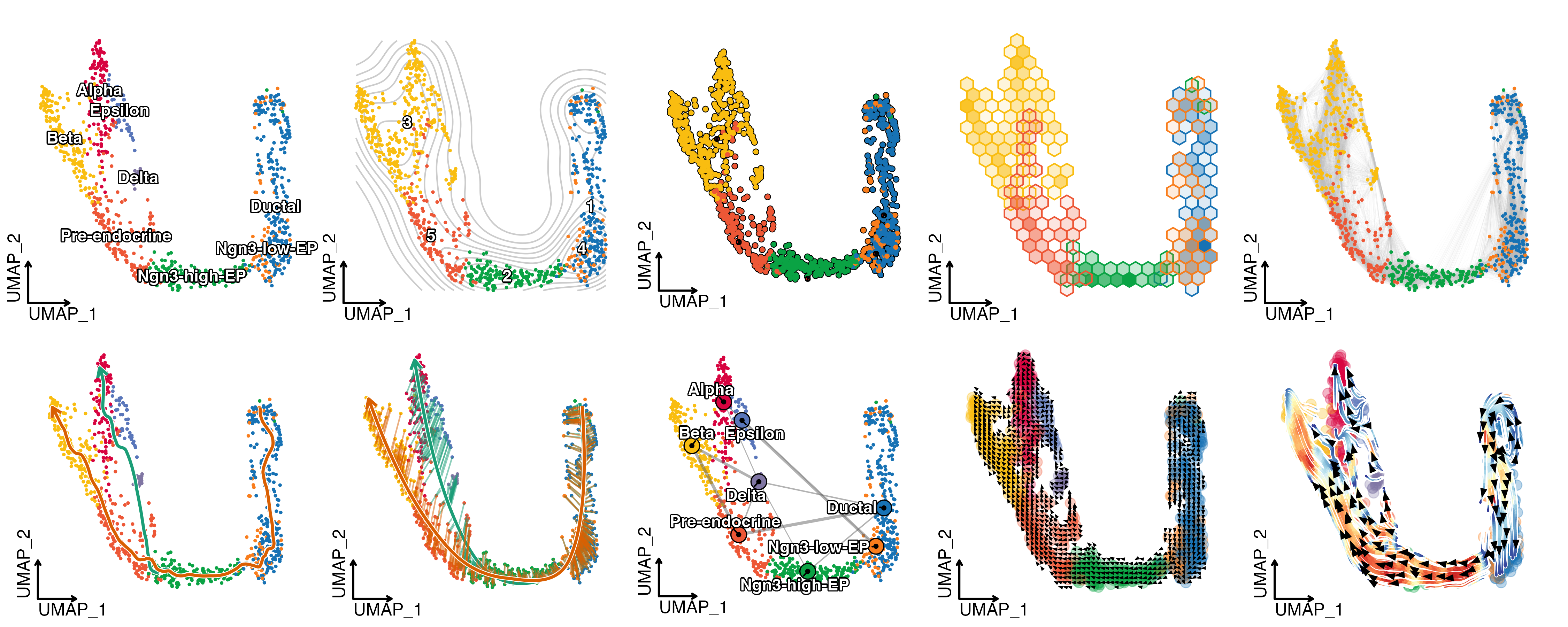
Trajectory inference
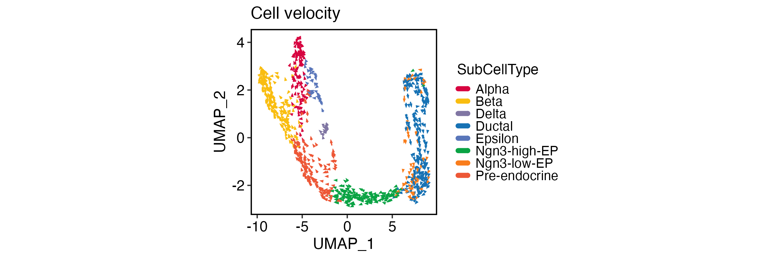
RNA Velocity analysis
To estimate RNA velocity, both “spliced” and “unspliced” assays are required in the Seurat object. You can generate these matrices using velocyto, bustools, or alevin.
pancreas_sub <- RunSCVELO(
  pancreas_sub,
  group.by = "SubCellType",
  linear_reduction = "PCA",
  nonlinear_reduction = "UMAP"
)
VelocityPlot(
  pancreas_sub,
  reduction = "UMAP",
  group.by = "SubCellType",
  xlab = "UMAP_1",
  ylab = "UMAP_2"
)
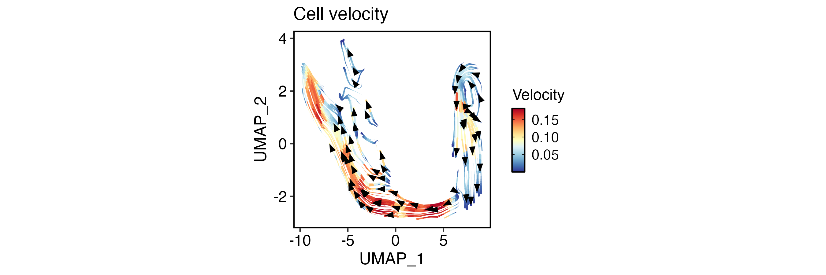
VelocityPlot(
  pancreas_sub,
  reduction = "UMAP",
  plot_type = "stream",
  xlab = "UMAP_1",
  ylab = "UMAP_2"
)
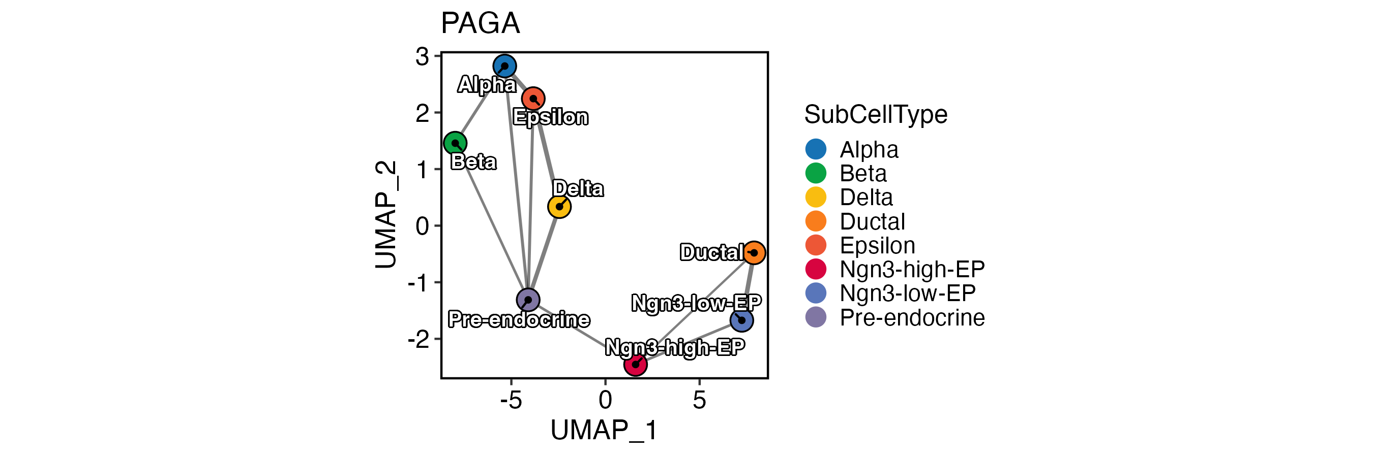
PAGA
pancreas_sub <- RunPAGA(
  pancreas_sub,
  group.by = "SubCellType",
  linear_reduction = "PCA",
  nonlinear_reduction = "UMAP"
)
PAGAPlot(
  pancreas_sub,
  reduction = "UMAP",
  label = TRUE,
  label_insitu = TRUE,
  label_repel = TRUE,
  edge_size = c(0.5, 1),
  edge_color = "black",
  xlab = "UMAP_1",
  ylab = "UMAP_2"
)
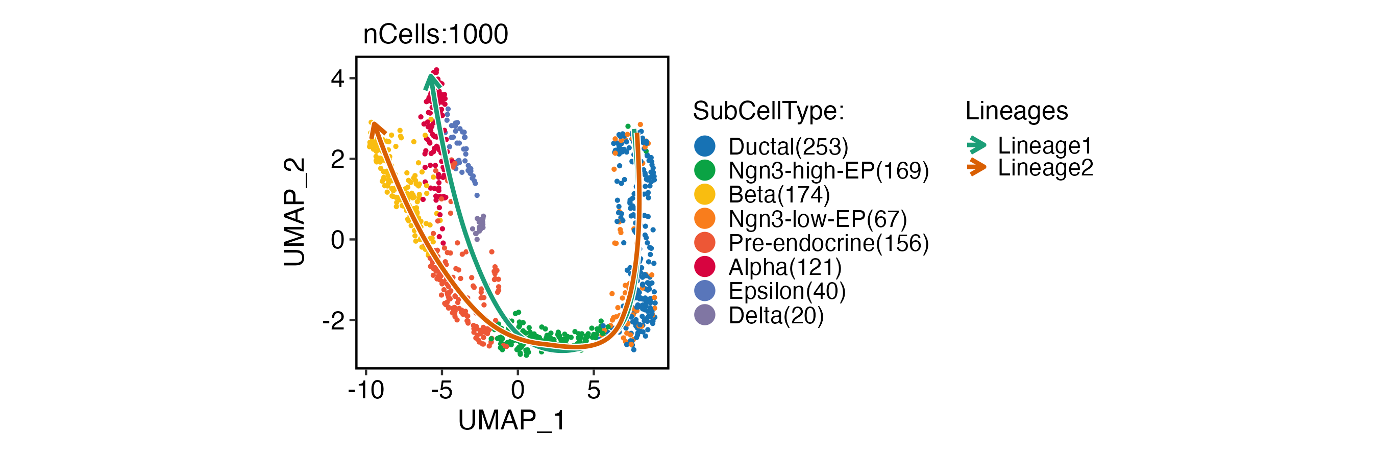
Slingshot
pancreas_sub <- RunSlingshot(
  pancreas_sub,
  group.by = "SubCellType",
  reduction = "UMAP",
  start = "Ductal",
  end = c("Alpha", "Beta")
)
CellDimPlot(
  pancreas_sub,
  group.by = "SubCellType",
  lineages = paste0("Lineage", 1:2),
  reduction = "UMAP",
  xlab = "UMAP_1",
  ylab = "UMAP_2"
)
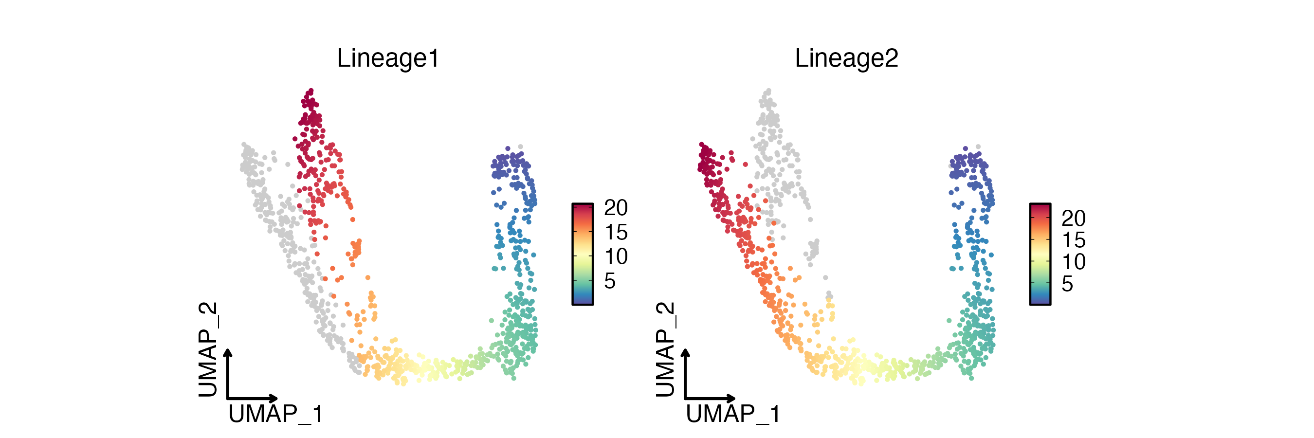
FeatureDimPlot(
  pancreas_sub,
  features = paste0("Lineage", 1:2),
  reduction = "UMAP",
  theme_use = "theme_blank",
  xlab = "UMAP_1",
  ylab = "UMAP_2"
)
Monocle3
pancreas_sub <- RunMonocle3(
  pancreas_sub,
  group.by = "SubCellType"
)
trajectory <- pancreas_sub@tools$Monocle3$trajectory
milestones <- pancreas_sub@tools$Monocle3$milestones
CellDimPlot(
  pancreas_sub,
  group.by = "Monocle3_partitions",
  reduction = "UMAP",
  label = TRUE,
  xlab = "UMAP_1",
  ylab = "UMAP_2"
) +
  trajectory +
  milestones +
  CellDimPlot(
    pancreas_sub,
    group.by = "Monocle3_clusters",
    reduction = "UMAP",
    label = TRUE,
    xlab = "UMAP_1",
    ylab = "UMAP_2"
  ) +
  trajectory +
  CellDimPlot(
    pancreas_sub,
    group.by = "SubCellType",
    reduction = "UMAP",
    label = TRUE,
    xlab = "UMAP_1",
    ylab = "UMAP_2"
  ) +
  trajectory +
  FeatureDimPlot(
    pancreas_sub,
    features = "Monocle3_Pseudotime",
    reduction = "UMAP",
    xlab = "UMAP_1",
    ylab = "UMAP_2"
  ) +
  trajectory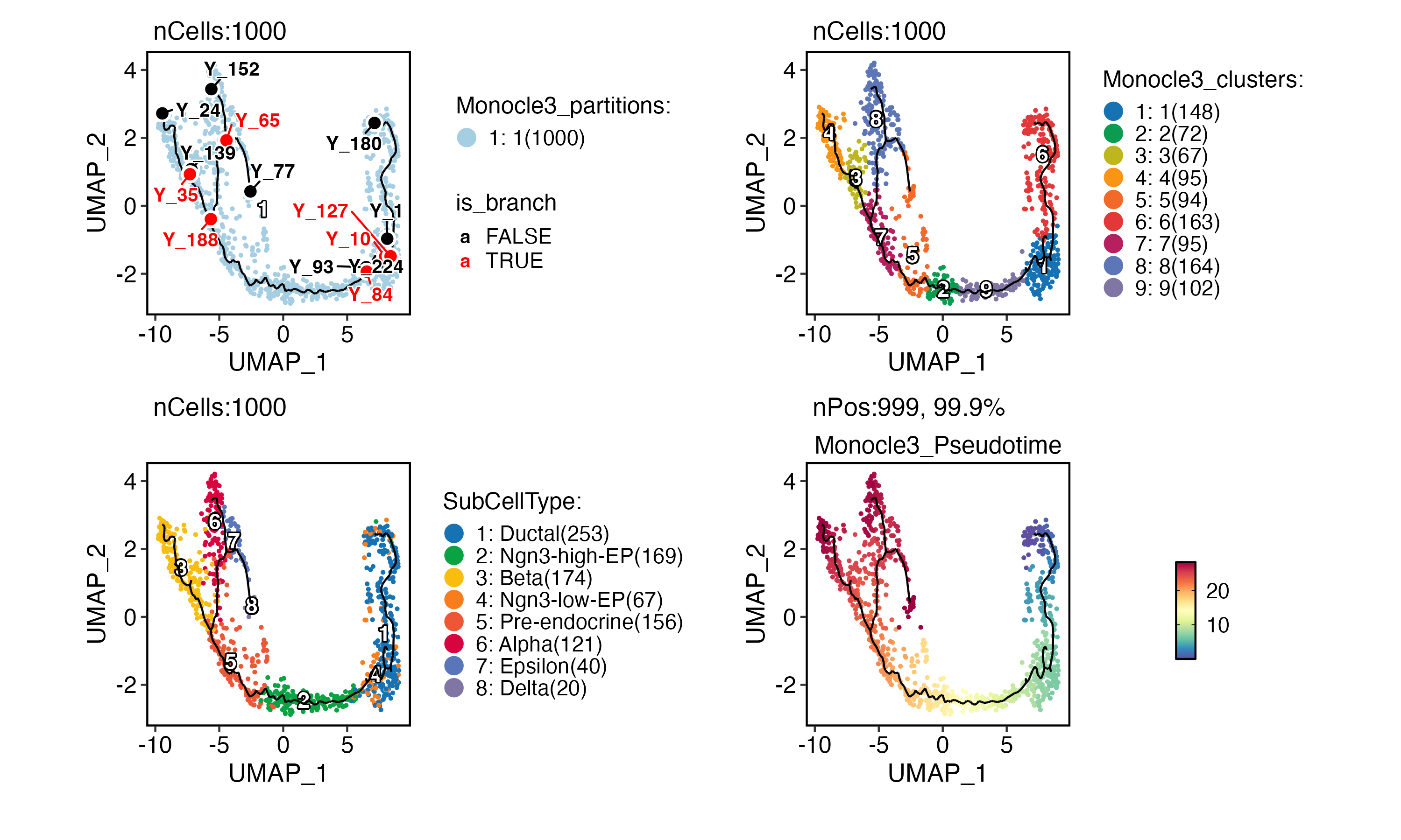
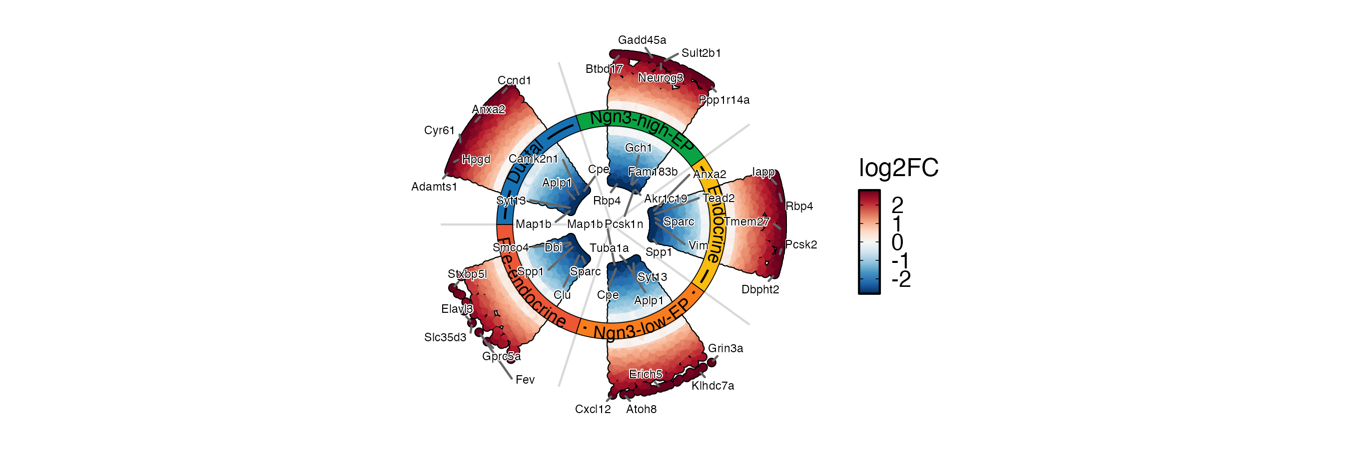
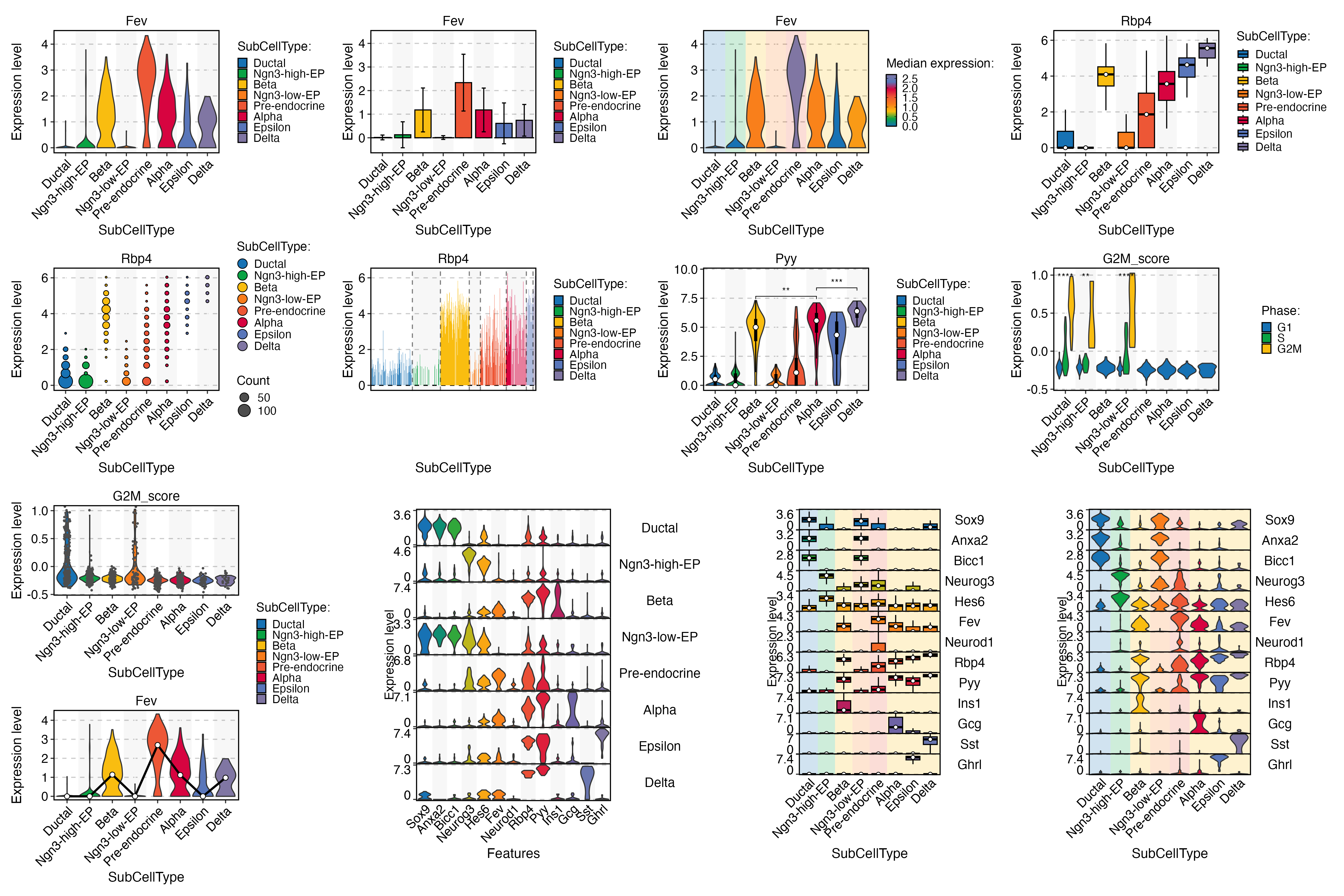
Dynamic features
pancreas_sub <- RunDynamicFeatures(
  pancreas_sub,
  lineages = c("Lineage1", "Lineage2"),
  n_candidates = 200
)
# Annotate features with transcription factors and surface proteins
pancreas_sub <- AnnotateFeatures(
  pancreas_sub,
  species = "Mus_musculus",
  db = c("TF", "CSPA")
)
ht <- DynamicHeatmap(
  pancreas_sub,
  lineages = c("Lineage1", "Lineage2"),
  use_fitted = TRUE,
  n_split = 6,
  reverse_ht = "Lineage1",
  species = "Mus_musculus",
  db = "GO_BP",
  anno_terms = TRUE,
  anno_keys = TRUE,
  anno_features = TRUE,
  exp_legend_title = "Z-score",
  heatmap_palette = "viridis",
  cell_annotation = "SubCellType",
  separate_annotation = list(
    "SubCellType", c("Nnat", "Irx1")
  ),
  separate_annotation_palette = c("Chinese", "Set1"),
  feature_annotation = c("TF", "CSPA"),
  feature_annotation_palcolor = list(
    c("gold", "steelblue"), c("forestgreen")
  ),
  pseudotime_label = 25,
  pseudotime_label_color = "red",
  cores = 6,
  height = 5,
  width = 2
)
print(ht$plot)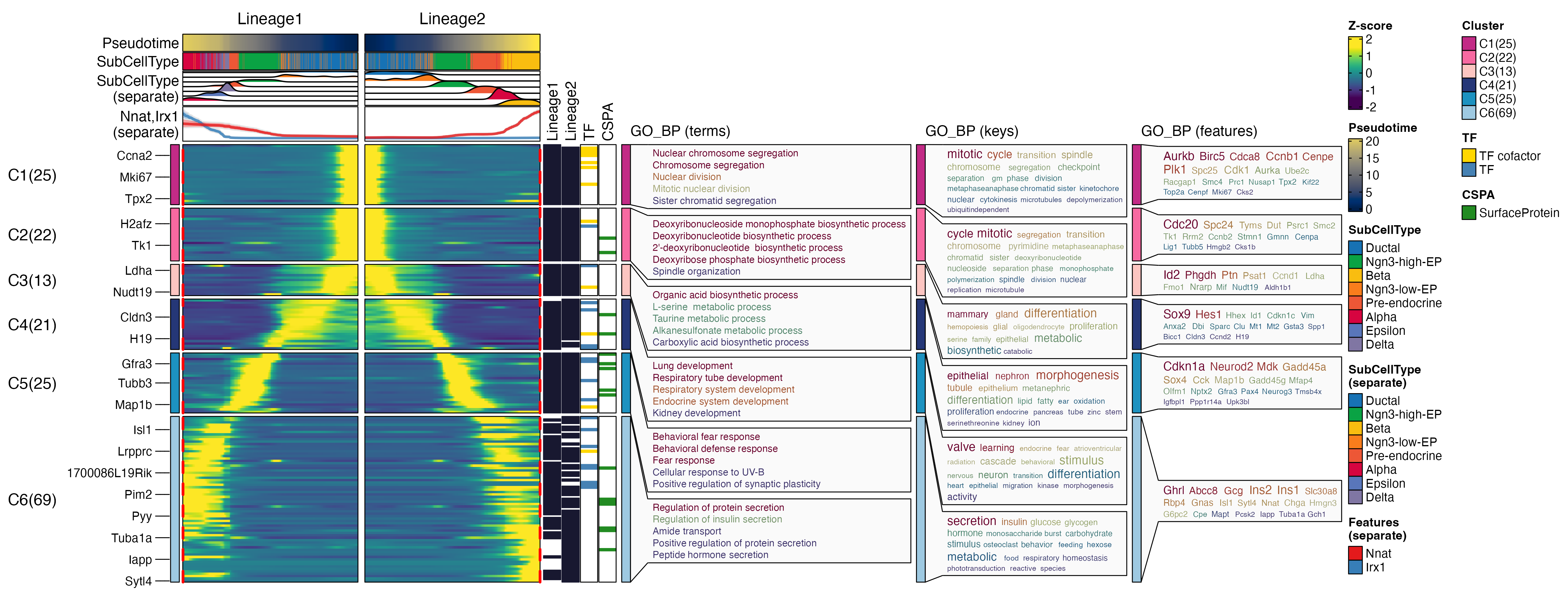
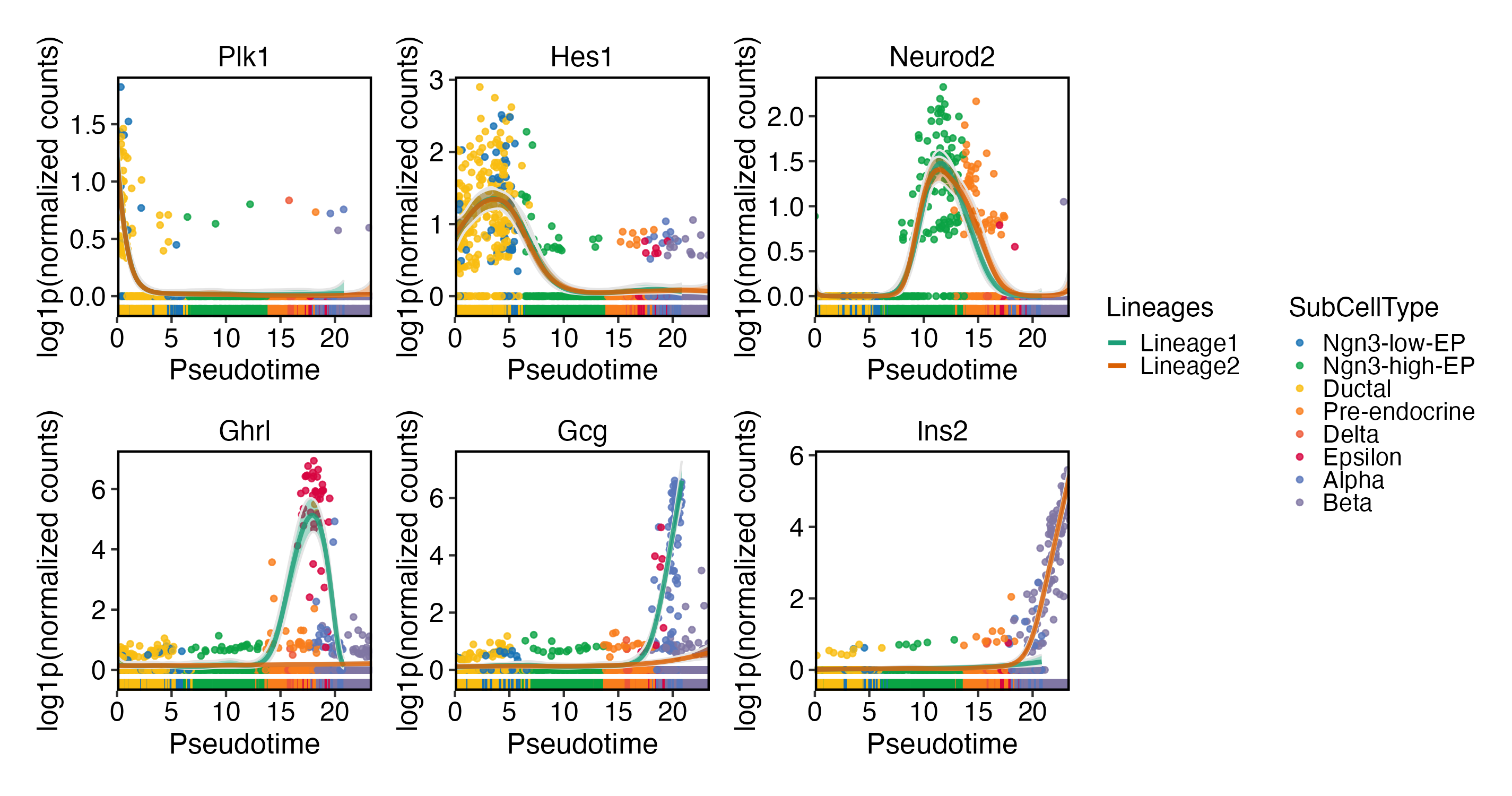
DynamicPlot(
  pancreas_sub,
  lineages = c("Lineage1", "Lineage2"),
  group.by = "SubCellType",
  features = c(
    "Plk1", "Hes1", "Neurod2",
    "Ghrl", "Gcg", "Ins2"
  )
)
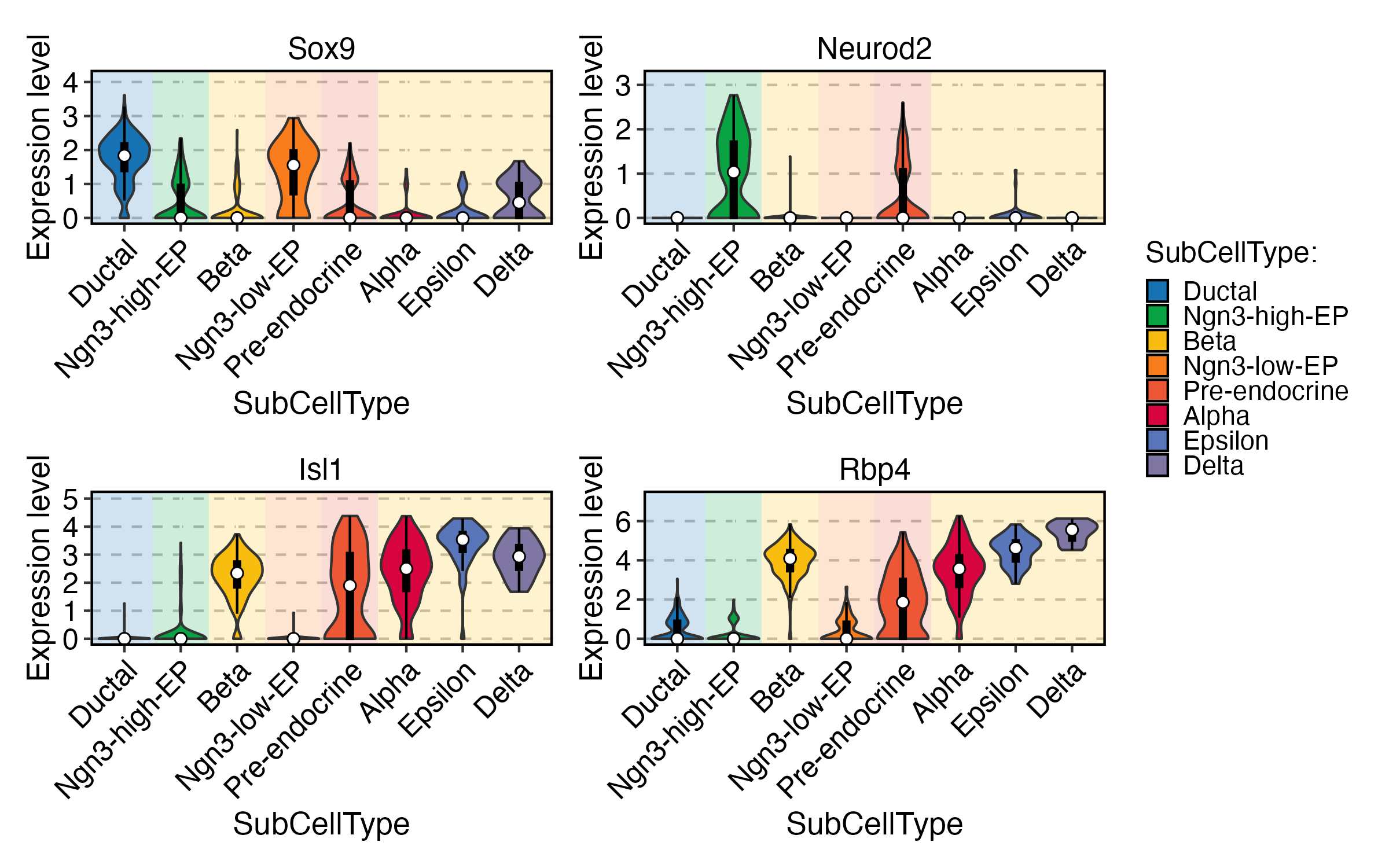
FeatureStatPlot(
  pancreas_sub,
  group.by = "SubCellType",
  bg.by = "CellType",
  stat.by = c("Sox9", "Neurod2", "Isl1", "Rbp4"),
  add_box = TRUE,
  comparisons = list(
    c("Ductal", "Ngn3 low EP"),
    c("Ngn3 high EP", "Pre-endocrine"),
    c("Alpha", "Beta")
  )
) + patchwork::plot_layout(
  guides = "collect"
)
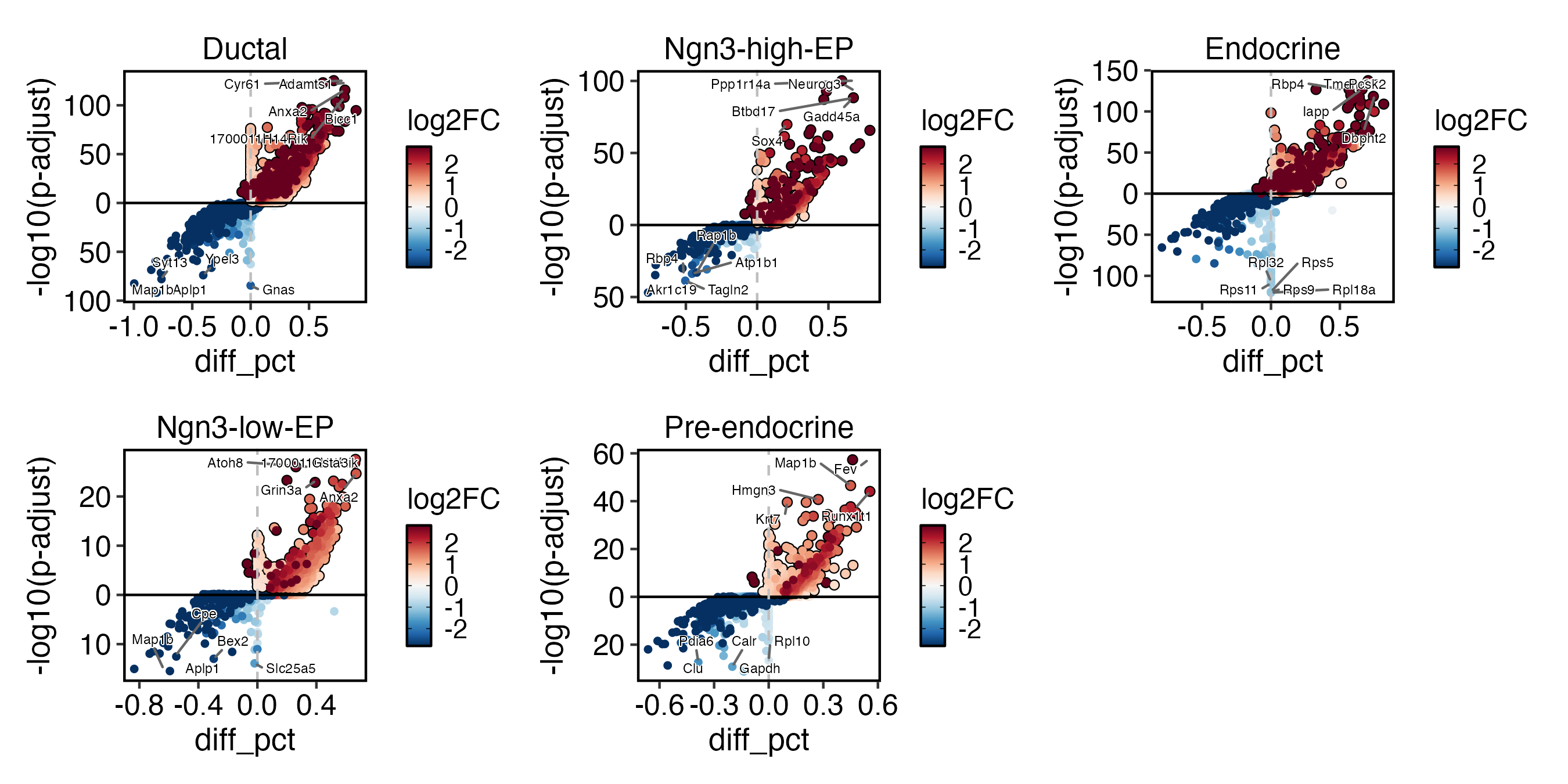
Differential expression analysis
pancreas_sub <- RunDEtest(
  pancreas_sub,
  group.by = "CellType",
  fc.threshold = 1,
  only.pos = FALSE
)
DEtestPlot(
  pancreas_sub,
  group.by = "CellType",
  plot_type = "volcano",
  label.size = 2
)
DEtestPlot(
  pancreas_sub,
  group.by = "CellType",
  plot_type = "manhattan",
  label.size = 2
) + ggplot2::theme(aspect.ratio = 1 / 2)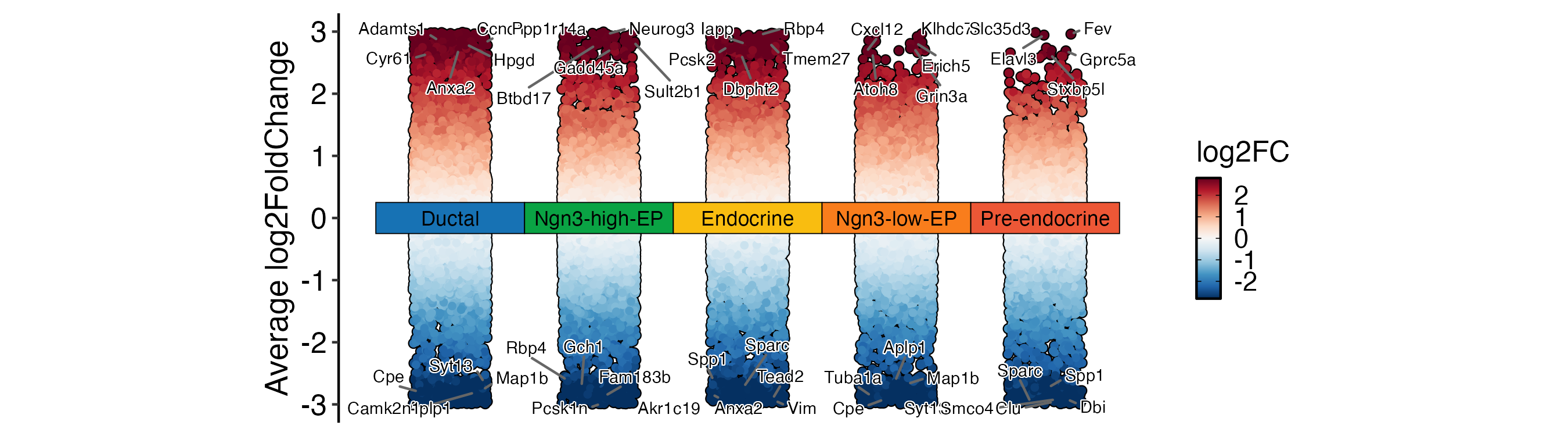
DEtestPlot(
  pancreas_sub,
  group.by = "CellType",
  plot_type = "ring",
  label.size = 2
)
DEGs <- pancreas_sub@tools$DEtest_CellType$AllMarkers_wilcox
DEGs <- DEGs[with(DEGs, avg_log2FC > 1 & p_val_adj < 0.05), ]

ht <- FeatureHeatmap(
  pancreas_sub,
  group.by = "CellType",
  features = DEGs$gene,
  feature_split = DEGs$group1,
  exp_legend_title = "Z-score",
  species = "Mus_musculus",
  db = c("GO_BP", "KEGG", "WikiPathway"),
  anno_terms = TRUE,
  feature_annotation = c("TF", "CSPA"),
  feature_annotation_palcolor = list(
    c("gold", "steelblue"), c("forestgreen")
  ),
  cores = 6,
  height = 5,
  width = 3
)
print(ht$plot)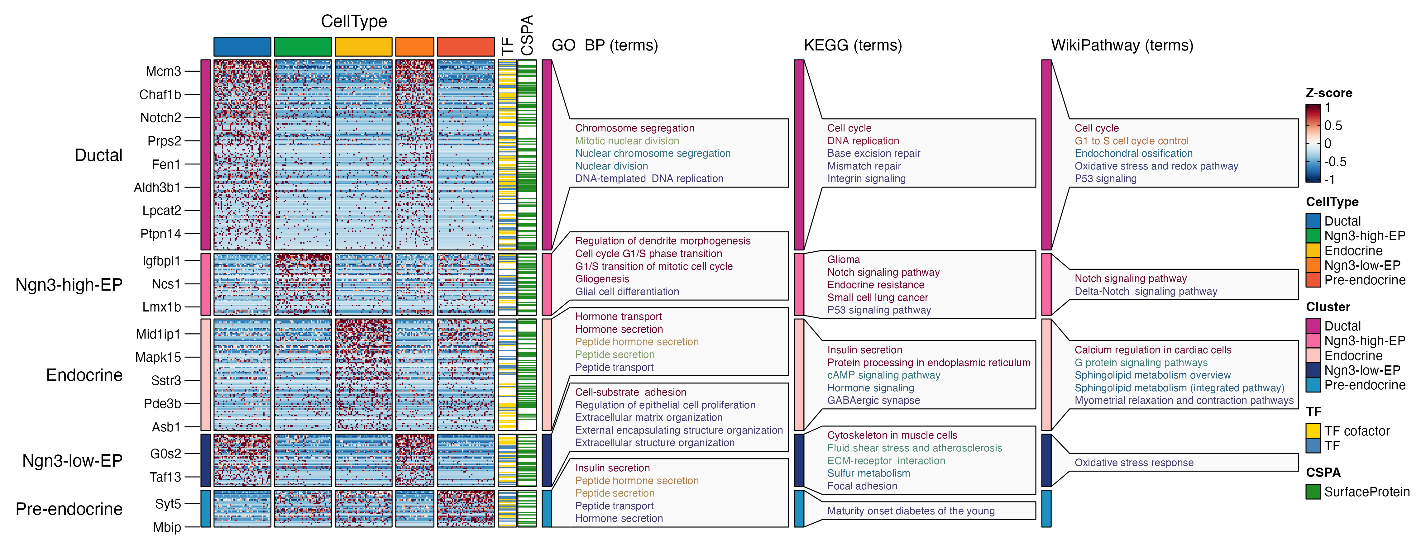
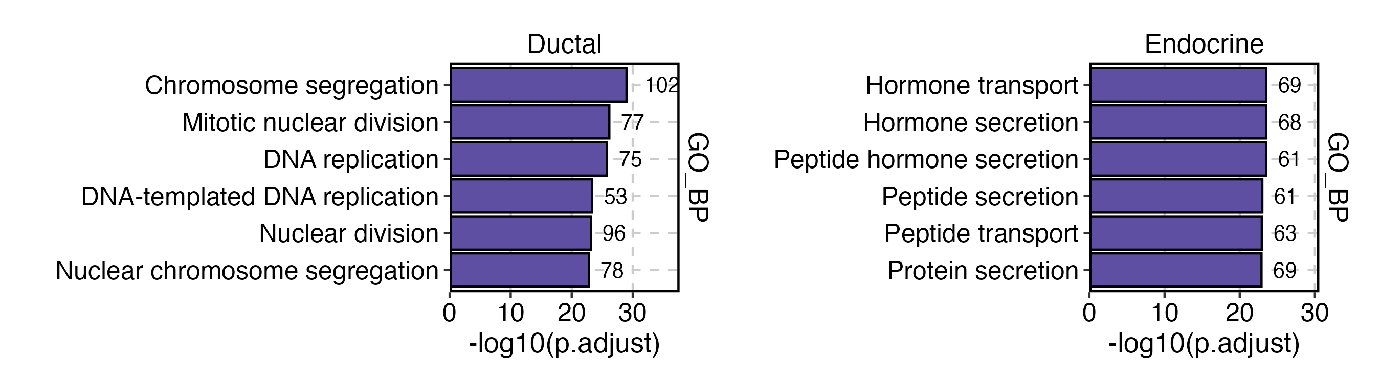
Enrichment analysis
Over-representation
pancreas_sub <- RunEnrichment(
pancreas_sub,
group.by = "CellType",
db = "GO_BP",
species = "Mus_musculus",
DE_threshold = "avg_log2FC > log2(1.5) & p_val_adj < 0.05",
cores = 5
)
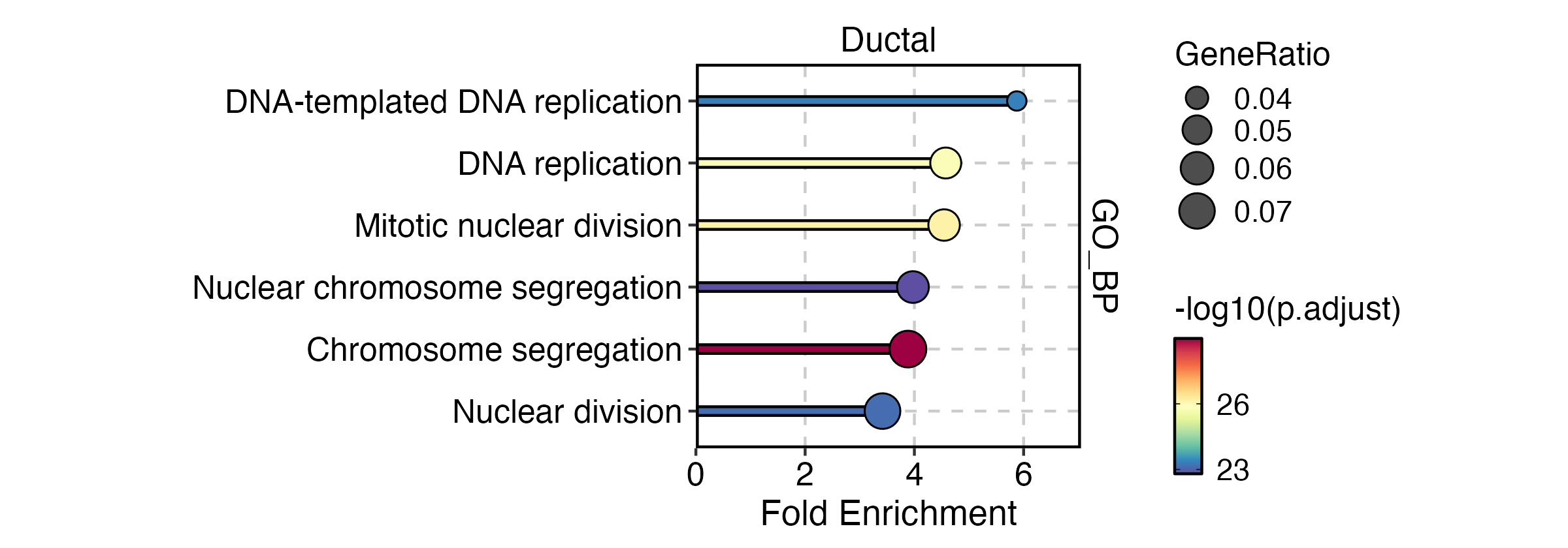
EnrichmentPlot(
pancreas_sub,
group.by = "CellType",
group_use = c("Ductal", "Endocrine"),
plot_type = "bar"
)
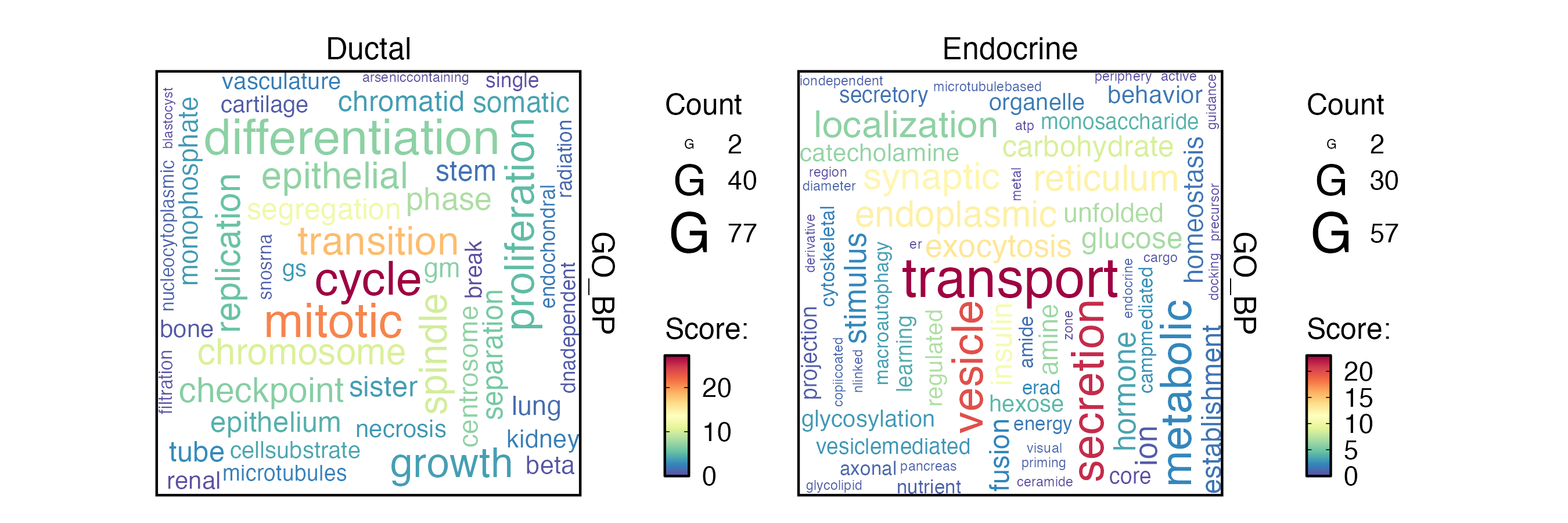
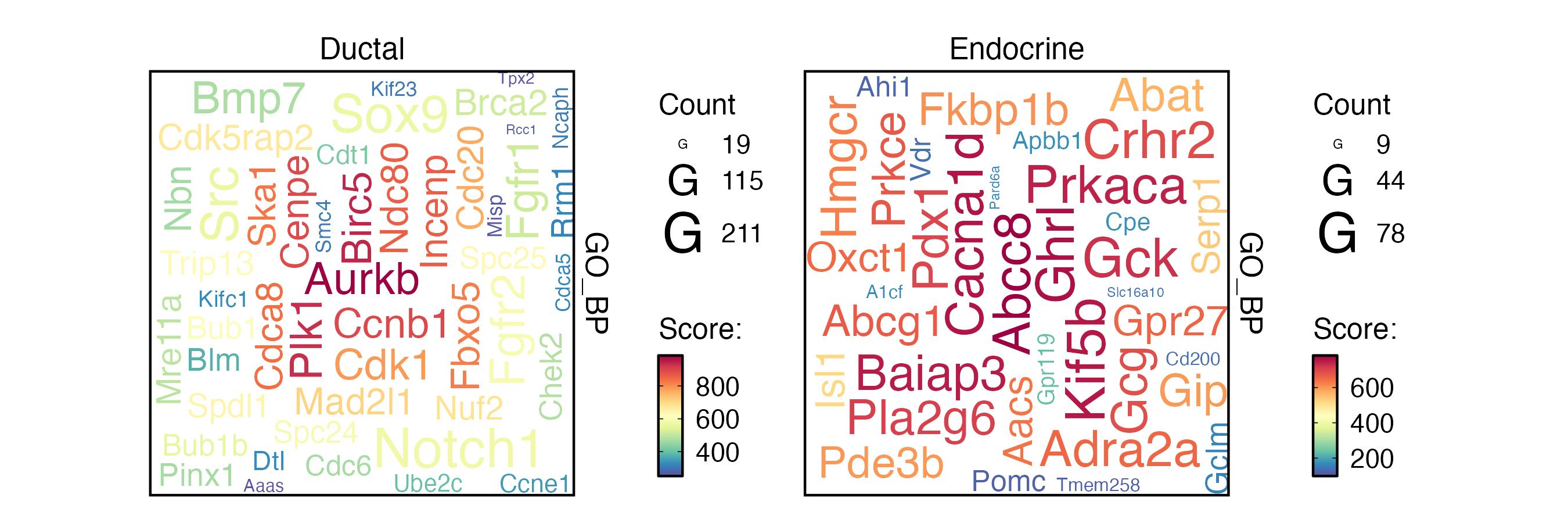
EnrichmentPlot(
  pancreas_sub,
  group.by = "CellType",
  group_use = c("Ductal", "Endocrine"),
  plot_type = "wordcloud"
)
EnrichmentPlot(
  pancreas_sub,
  group.by = "CellType",
  group_use = c("Ductal", "Endocrine"),
  plot_type = "wordcloud",
  word_type = "feature"
)
EnrichmentPlot(
  pancreas_sub,
  group.by = "CellType",
  group_use = "Ngn3-low-EP",
  plot_type = "network"
)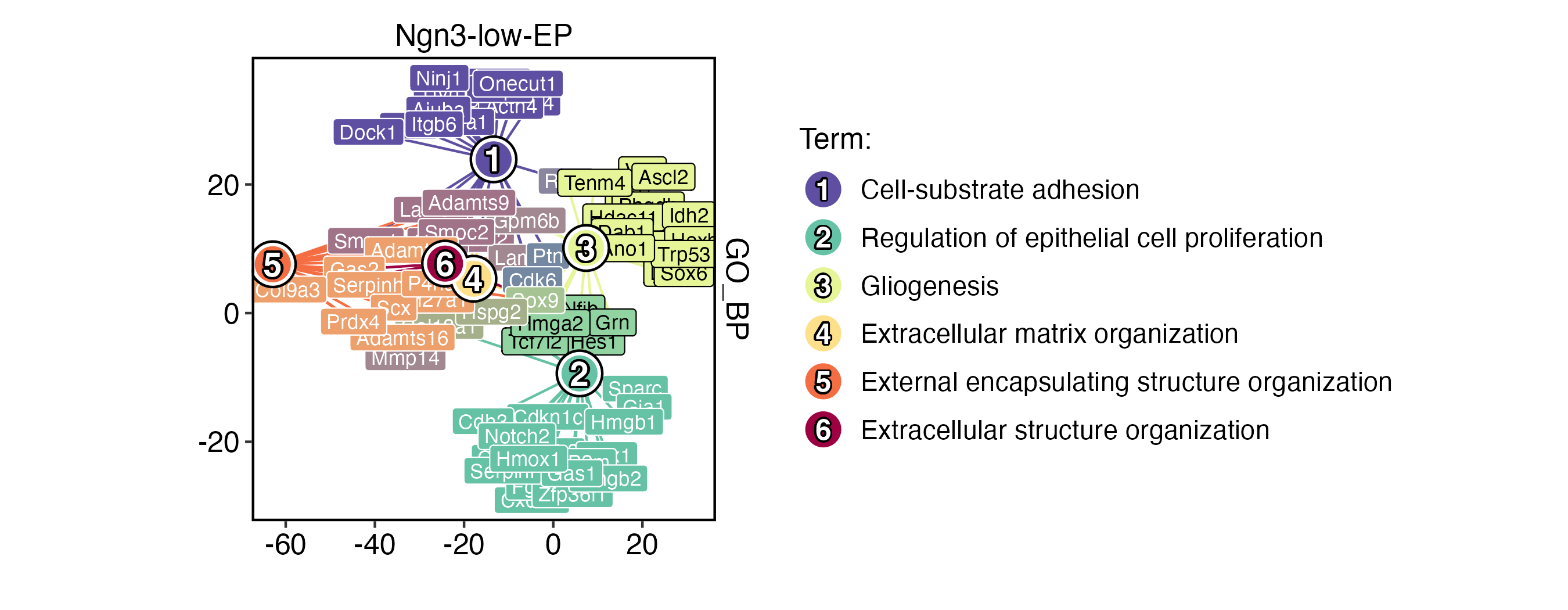
To ensure that labels are visible, you can adjust the size of the viewer panel on Rstudio IDE.
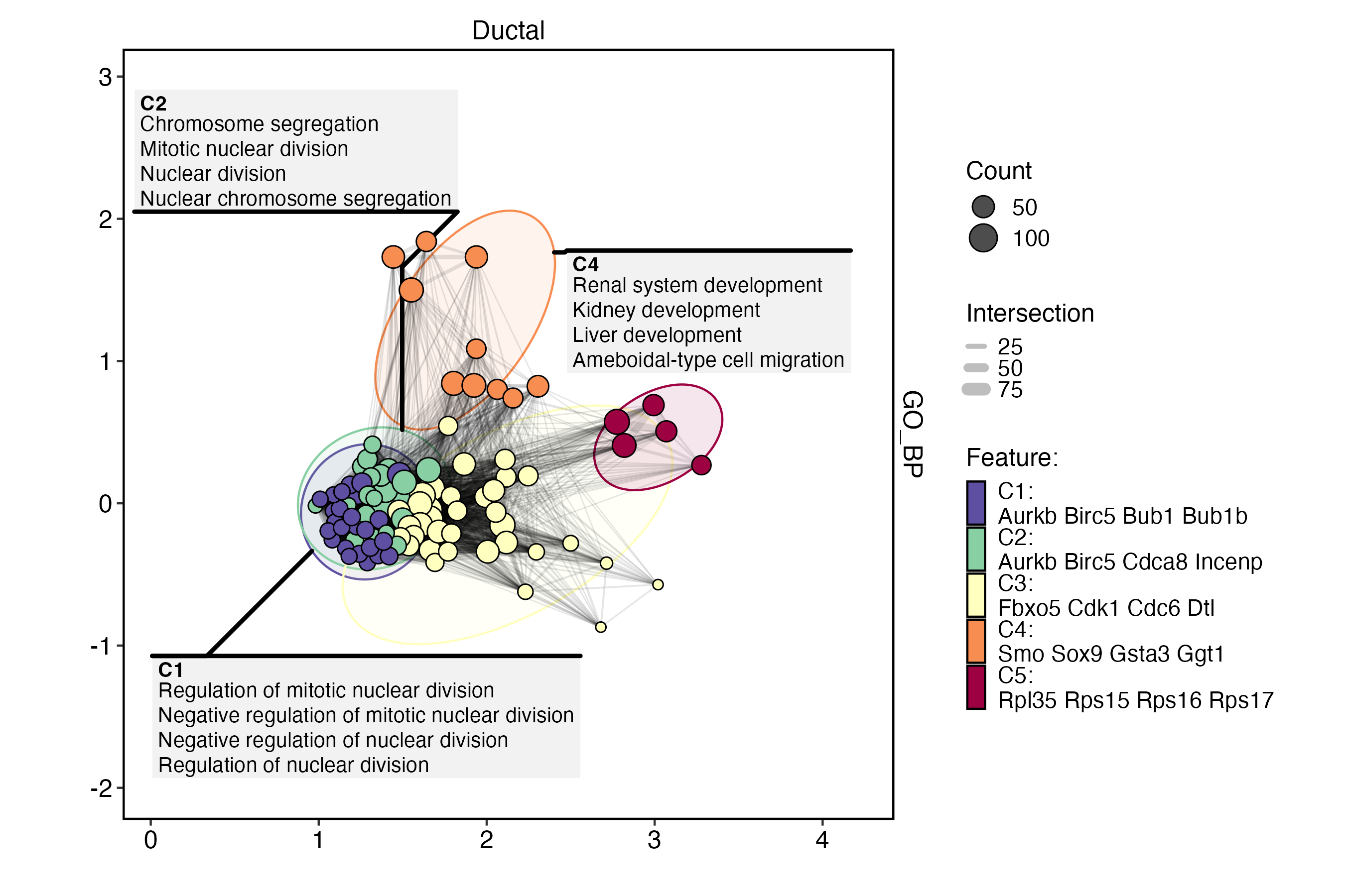
EnrichmentPlot(
  pancreas_sub,
  group.by = "CellType",
  group_use = "Ductal",
  plot_type = "enrichmap"
)
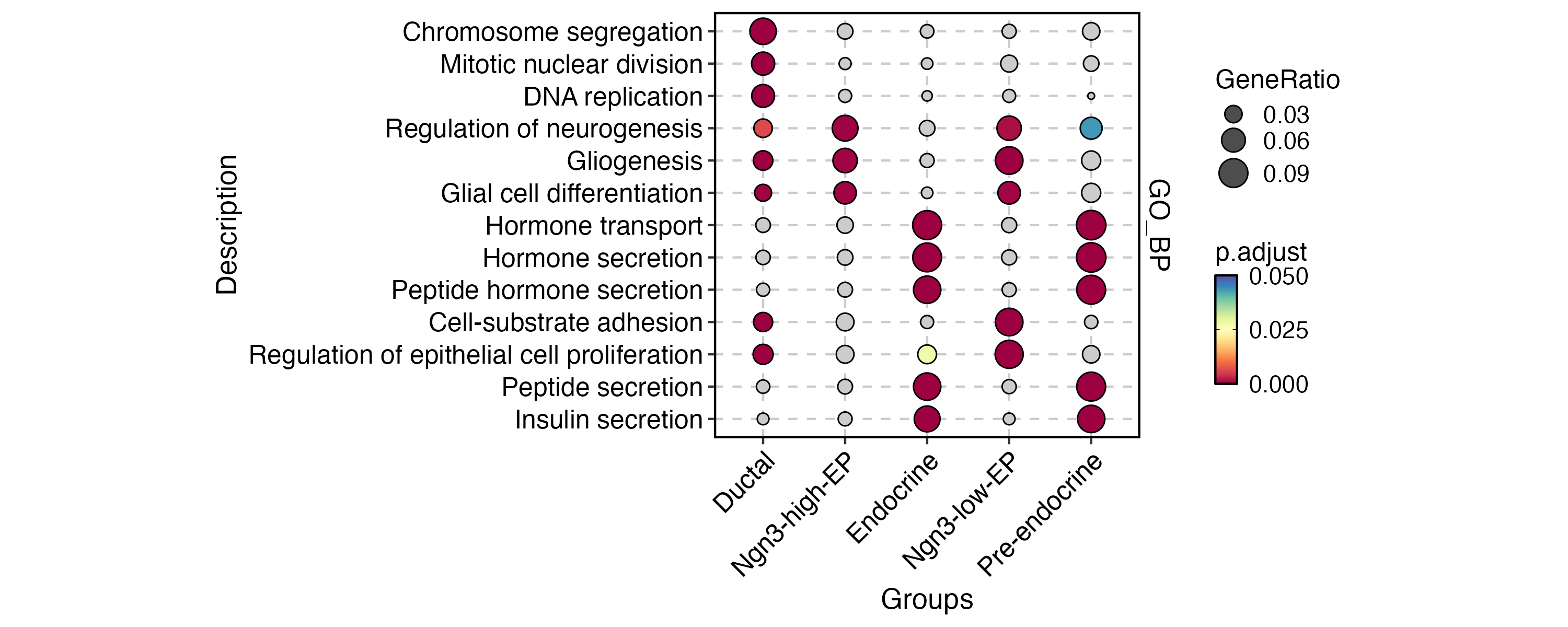
EnrichmentPlot(
  pancreas_sub,
  group.by = "CellType",
  plot_type = "comparison",
  topTerm = 3
)
EnrichmentPlot(
  pancreas_sub,
  group.by = "CellType",
  group_use = "Ductal",
  plot_type = "lollipop"
)
GSEA
pancreas_sub <- RunGSEA(
pancreas_sub,
group.by = "CellType",
db = "GO_BP",
species = "Mus_musculus",
DE_threshold = "p_val_adj < 0.05",
cores = 5
)
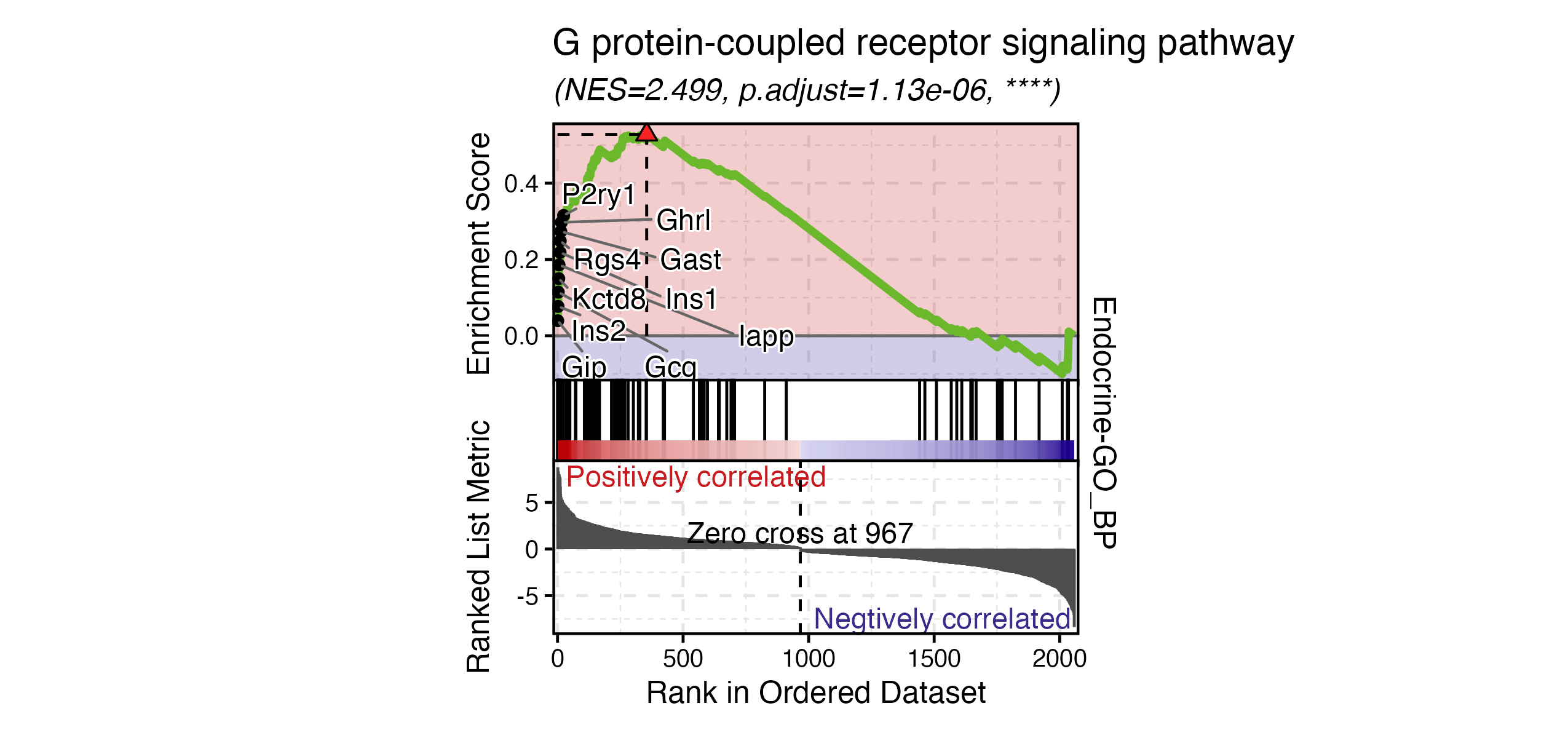
GSEAPlot(
pancreas_sub,
group.by = "CellType",
group_use = "Endocrine",
id_use = "GO:0007186"
)
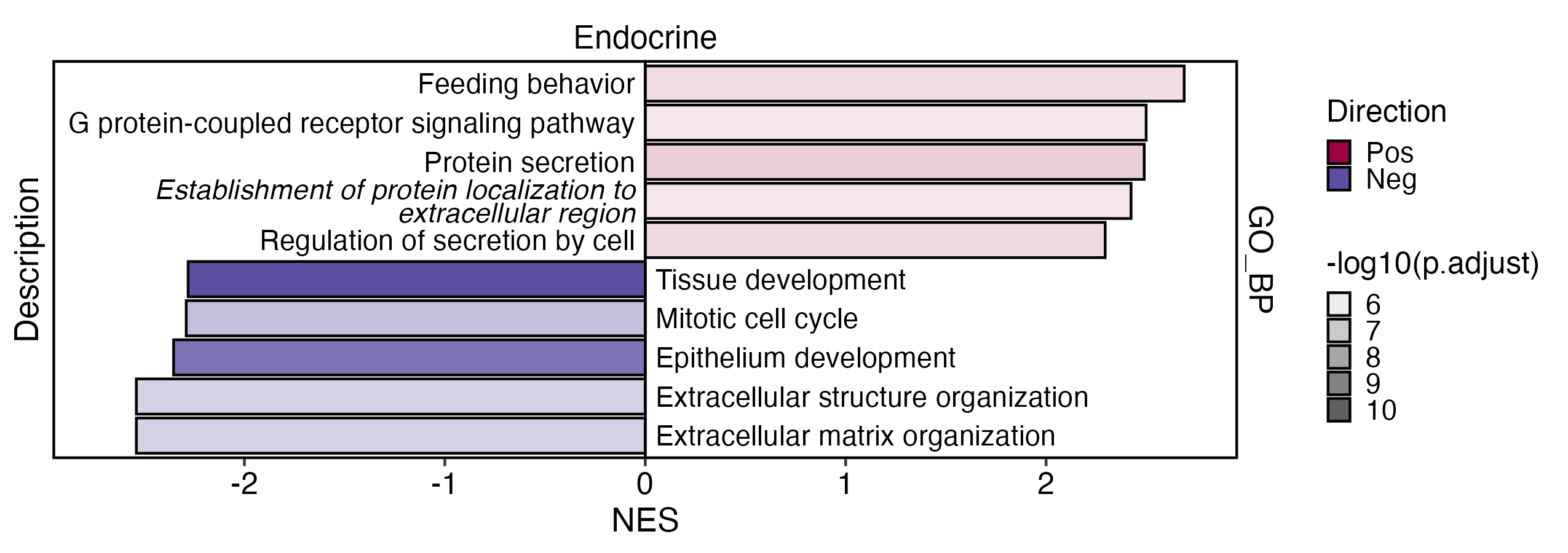
GSEAPlot(
  pancreas_sub,
  group.by = "CellType",
  group_use = "Endocrine",
  plot_type = "bar",
  direction = "both",
  topTerm = 10
)
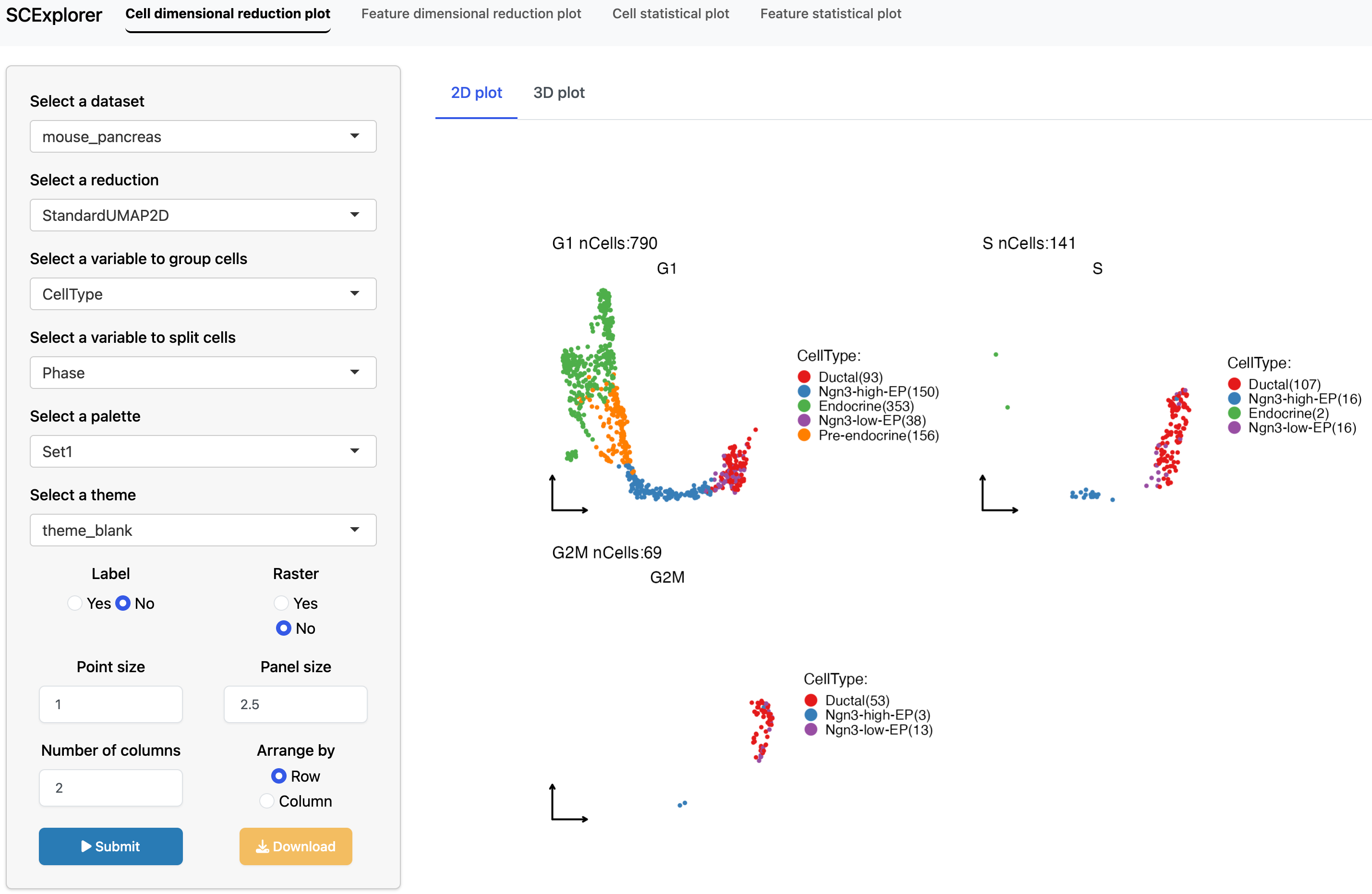
Interactive data visualization with SCExplorer
PrepareSCExplorer(
  list(
    mouse_pancreas = pancreas_sub,
    human_pancreas = panc8_sub
  ),
  base_dir = "./SCExplorer"
)
app <- RunSCExplorer(base_dir = "./SCExplorer")
list.files("./SCExplorer") # This directory can be used as site directory for Shiny Server.

if (interactive()) {
  shiny::runApp(app)
}
Other visualization examples
You can also find more examples in the documentation of the function: integration_scop, RunKNNMap, RunPalantir, etc.