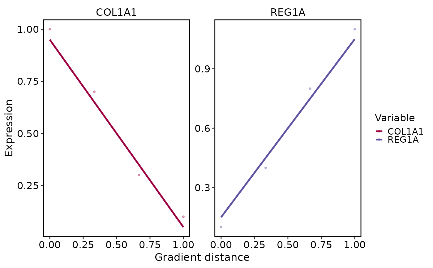
Plot spatial gradient screening results — SpatialGradientPlot • scop

Visualize normalized results produced by RunSpatialGradientFeatures() without requiring the original SPATA2 object.

Usage

SpatialGradientPlot(
  srt,
  result_name = NULL,
  plot_type = c("summary", "surface", "line", "model", "combined"),
  features = NULL,
  nfeatures = 4,
  assay = NULL,
  layer = "data",
  image = NULL,
  overlay_image = TRUE,
  image.alpha = 1,
  coord.cols = c("col", "row"),
  flip.y = TRUE,
  pt.size = NULL,
  pt.alpha = 0.9,
  stroke = 0.1,
  palette = "Spectral",
  palcolor = NULL,
  legend.position = "right",
  theme_use = "theme_scop",
  theme_args = list(),
  line_size = 1,
  line_alpha = 0.35,
  line_fit = c("stored", "lm"),
  nrow = NULL,
  ncol = NULL,
  byrow = TRUE
)

Arguments

srt: A Seurat object.
result_name: Stored spatial gradient result name. If NULL, the latest stored result is used.
plot_type: Plot type: "summary", "surface", "line", "model", or "combined".
features: Variables to plot. If NULL, top variables from the stored result are used.
nfeatures: Number of top variables used when features = NULL.
assay: Assay used for features. If NULL, the default assay is used.
layer: Assay layer used for features.
image: Name of the Seurat spatial image. If NULL, the first image is used when present.
overlay_image: Whether to draw the spatial image beneath spots.
image.alpha: Transparency of the spatial image.
coord.cols: Metadata coordinate columns used when no image is available.
flip.y: Whether to reverse the y axis for metadata coordinates.
pt.size: Point size.
pt.alpha: Point alpha.
stroke: Point border width.
palette, palcolor: Color palette passed to SCOP plotting helpers.
legend.position: The position of legends, one of "none", "left", "right", "bottom", "top". Default is "right".
theme_use: Theme used. Can be a character string or a theme function. Default is "theme_scop".
theme_args: Other arguments passed to the theme_use. Default is list().
line_size: Size of fitted gradient lines.
line_alpha: Alpha for raw value points.
line_fit: Gradient line source. "stored" uses the saved screening$estimate values produced by the selected backend. "lm" draws a fresh linear fit from screening$value, which is useful for showing a simple monotonic trend even when the backend stores a smoothed curve.
nrow: Number of rows in the combined plot. Default is NULL, which means determined automatically based on the number of plots.
ncol: Number of columns in the combined plot. Default is NULL, which means determined automatically based on the number of plots.
byrow: Whether to arrange the plots by row in the combined plot. Default is TRUE.

Value

A ggplot or patchwork object.

Examples

counts <- matrix(
  c(4, 1, 0, 2, 1, 3, 2, 0),
  nrow = 2,
  byrow = TRUE
)
rownames(counts) <- c("REG1A", "COL1A1")
colnames(counts) <- paste0("spot", 1:4)
srt <- Seurat::CreateSeuratObject(counts)
#> Warning: Data is of class matrix. Coercing to dgCMatrix.
srt <- Seurat::NormalizeData(srt, verbose = FALSE)
srt$col <- c(0, 1, 0, 1)
srt$row <- c(0, 0, 1, 1)

gradient_result <- list(
  screening = data.frame(
    variable = rep(c("REG1A", "COL1A1"), each = 4),
    distance = rep(seq(0, 1, length.out = 4), 2),
    value = c(0.1, 0.4, 0.8, 1.1, 1.0, 0.7, 0.3, 0.1),
    estimate = c(0.15, 0.45, 0.75, 1.05, 0.95, 0.65, 0.35, 0.05)
  ),
  significance = data.frame(
    variable = c("REG1A", "COL1A1"),
    p_value = c(0.004, 0.018),
    q_value = c(0.008, 0.024)
  ),
  model_fits = data.frame(
    variable = rep(c("REG1A", "COL1A1"), each = 2),
    model = rep(c("linear", "spline"), 2),
    rmse = c(0.12, 0.08, 0.18, 0.11)
  ),
  top_variables = data.frame(
    variable = c("REG1A", "COL1A1"),
    rank = 1:2,
    rmse = c(0.08, 0.11)
  ),
  parameters = data.frame(
    key = c("assay", "layer", "reference"),
    value = c("RNA", "data", "ductal_axis")
  )
)
srt@tools[["SpatialGradientFeatures"]] <- list(ductal_axis = gradient_result)
srt@misc[["SpatialGradientFeaturesResult"]] <- "ductal_axis"

SpatialGradientPlot(srt, plot_type = "summary", nfeatures = 2)

SpatialGradientPlot(srt, plot_type = "line", nfeatures = 2)

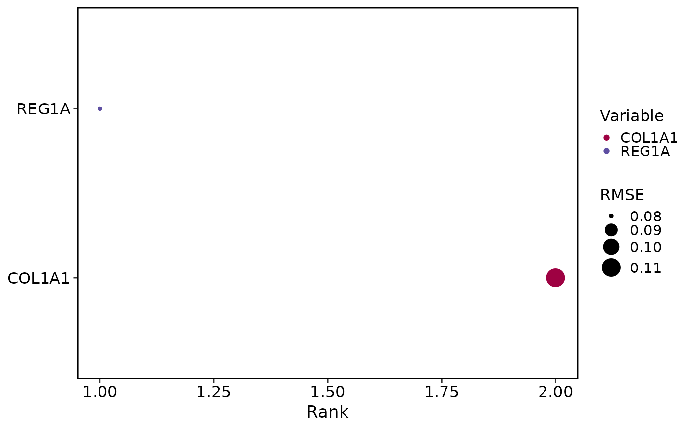SpatialGradientPlot(srt, plot_type = "model", nfeatures = 2)

SpatialGradientPlot(
  srt,
  plot_type = "surface",
  nfeatures = 2,
  overlay_image = FALSE,
  coord.cols = c("col", "row"),
  pt.size = 4
)