Plot Giotto backend results — GiottoPlot • scop

Plot standalone Giotto backend results with scop plotting conventions. The input Seurat object, when supplied, is copied internally for plotting and is not modified.

Usage

GiottoPlot(x, ...)

# S3 method for class 'giotto2_cluster'
GiottoPlot(
  x,
  srt,
  image = x$parameters$image %||% NULL,
  coord.cols = x$parameters$coord.cols %||% c("x", "y"),
  overlay_image = TRUE,
  crop = TRUE,
  pt.size = NULL,
  pt.alpha = 0.95,
  stroke = 0.08,
  palette = "Chinese",
  feature_palette = "Spectral",
  bg_color = "grey25",
  legend.position = "right",
  theme_use = "theme_blank",
  theme_args = list(),
  title = "Giotto Leiden clusters",
  subtitle = NULL,
  ...
)

# S3 method for class 'giotto2_cell_proximity'
GiottoPlot(
  x,
  heatmap_palette = "RdBu",
  heatmap_palcolor = NULL,
  theme_use = "theme_scop",
  theme_args = list(),
  title = "Giotto cell proximity enrichment",
  subtitle = NULL,
  ...
)

# S3 method for class 'giotto2_spatial_genes'
GiottoPlot(
  x,
  srt = NULL,
  plot_type = c("ranking", "feature"),
  feature = NULL,
  top_n = 20,
  assay = x$parameters$assay %||% NULL,
  layer = x$parameters$layer %||% "data",
  image = x$parameters$image %||% NULL,
  coord.cols = x$parameters$coord.cols %||% c("x", "y"),
  overlay_image = TRUE,
  crop = TRUE,
  pt.size = NULL,
  pt.alpha = 0.95,
  palette = "Chinese",
  feature_palette = "Spectral",
  heatmap_palette = "RdBu",
  heatmap_palcolor = NULL,
  legend.position = "right",
  theme_use = "theme_scop",
  theme_args = list(),
  title = NULL,
  subtitle = NULL,
  ...
)

# S3 method for class 'giotto2_spatial_modules'
GiottoPlot(
  x,
  features = NULL,
  top_n = 20,
  heatmap_palette = "RdBu",
  heatmap_palcolor = NULL,
  theme_use = "theme_scop",
  theme_args = list(),
  title = "Giotto spatial co-expression",
  subtitle = "Spatial correlation among top features",
  ...
)

Arguments

x: A result returned by one of the RunGiotto*() functions.
...: Arguments passed to S3 methods.
srt: Original `Seurat` object used to create the Giotto result. Required for spatial spot plots.
image: Name of the Seurat spatial image. If `NULL`, the first image is used when available.
coord.cols: Metadata coordinate columns used when no image is available.
overlay_image: Whether to draw the spatial image beneath spots.
crop: Whether to crop spatial panels to plotted spots.
pt.size: Point size for spatial plots.
pt.alpha: Point alpha for spatial plots.
stroke: Point border width for discrete spatial plots.
palette: Discrete palette used for groups.
feature_palette: Continuous palette used for spatial expression plots.
bg_color: Point border color for discrete spatial plots.
legend.position: Legend position.
theme_use: Theme function name used by scop plots.
theme_args: Additional arguments passed to `theme_use`.
title, subtitle: Plot title and subtitle. If `NULL`, sensible defaults are used.
heatmap_palette: Continuous palette used for heatmaps.
heatmap_palcolor: Optional custom colors used to create `heatmap_palette`.
plot_type: Plot type for spatial gene results. `"ranking"` plots the feature-level table; `"feature"` plots expression of one feature on spatial coordinates.
feature: Feature to draw for `plot_type = "feature"`. If `NULL`, the top Giotto feature is used.
top_n: Number of rows shown in ranking plots.
assay: Assay used for spatial feature expression plots.
layer: Assay layer used for spatial feature expression plots.
features: Features used for spatial co-expression heatmaps. If `NULL`, top features from the Giotto result are used.

Value

A ggplot object.

Examples

data(visium_human_pancreas_sub)
spatial <- visium_human_pancreas_sub
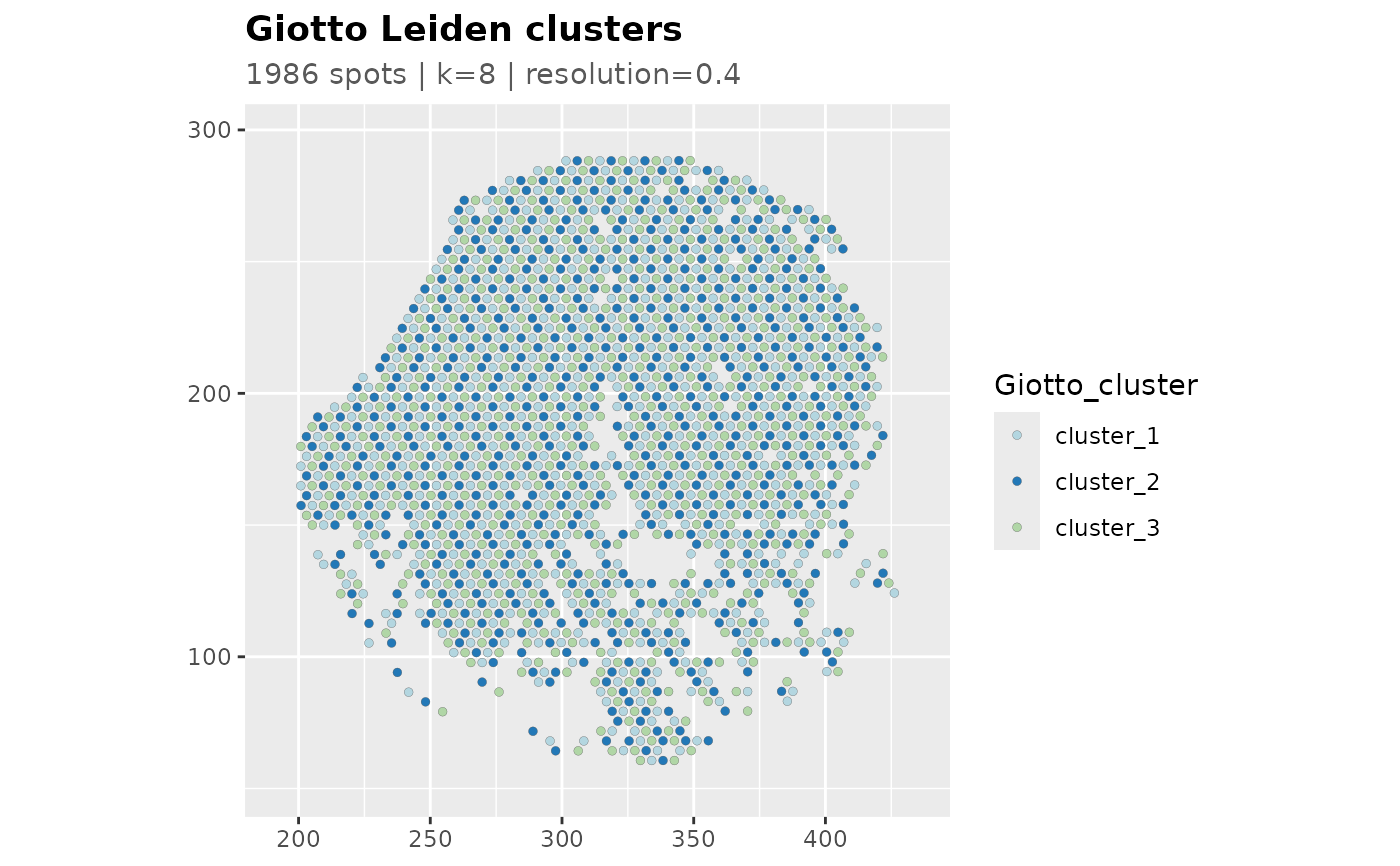
cluster_result <- list(
  clusters = data.frame(
    cluster = paste0("cluster_", (seq_len(ncol(spatial)) - 1) %% 3 + 1),
    row.names = colnames(spatial)
  ),
  parameters = list(
    cluster_colname = "Giotto_cluster",
    coord.cols = c("x", "y"),
    k = 8,
    resolution = 0.4
  )
)
class(cluster_result) <- c("giotto2_cluster", "giotto2_result", "list")
GiottoPlot(
  cluster_result,
  srt = spatial,
  overlay_image = FALSE,
  coord.cols = c("x", "y")
)


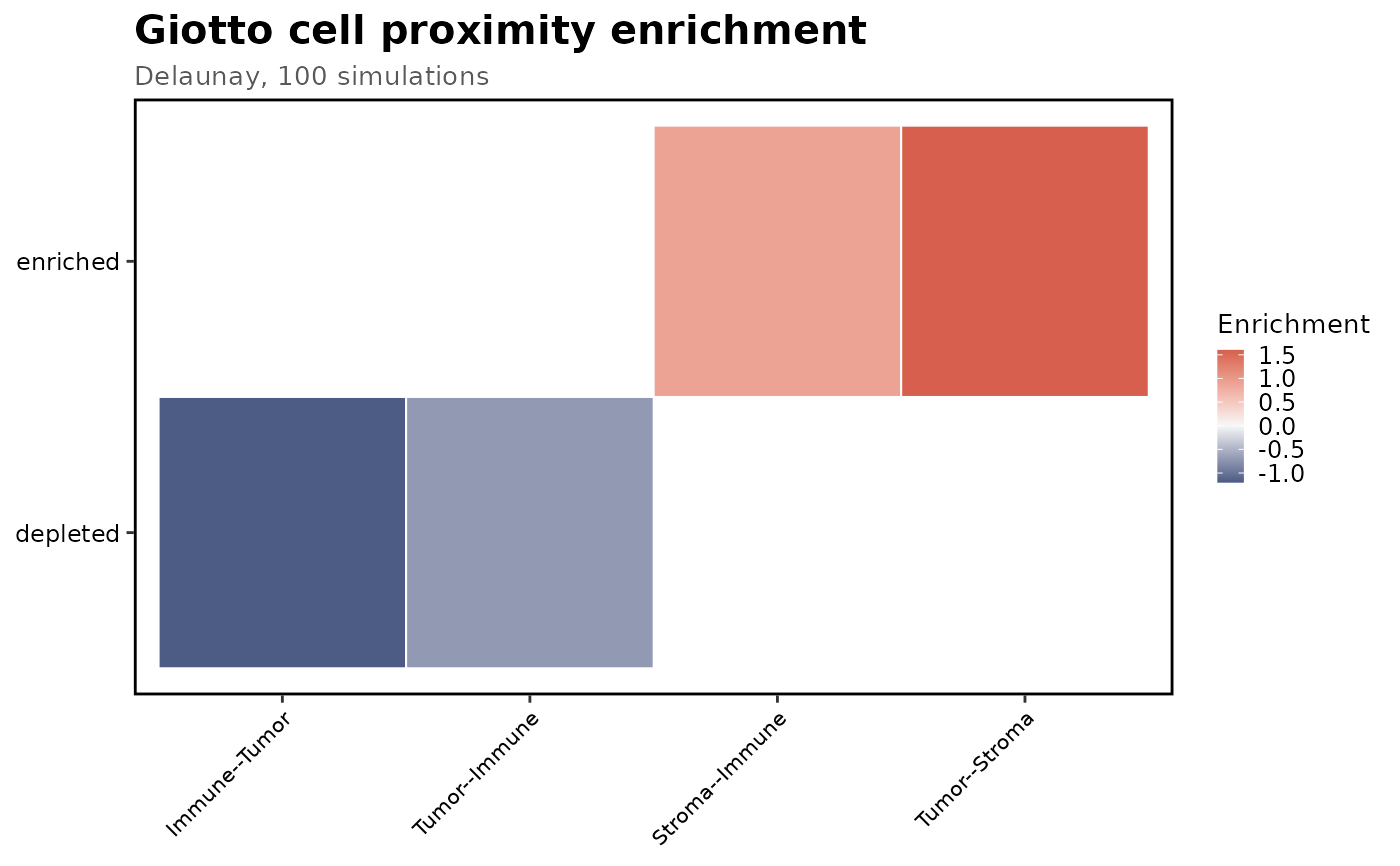
proximity <- list(
  enrichment = data.frame(
    group_1 = c("Tumor", "Tumor", "Stroma", "Immune"),
    group_2 = c("Stroma", "Immune", "Immune", "Tumor"),
    enrichment = c(1.6, -0.7, 0.9, -1.2),
    type_int = c("enriched", "depleted", "enriched", "depleted")
  ),
  parameters = list(network_method = "Delaunay", number_of_simulations = 100)
)
class(proximity) <- c("giotto2_cell_proximity", "giotto2_result", "list")
GiottoPlot(proximity)


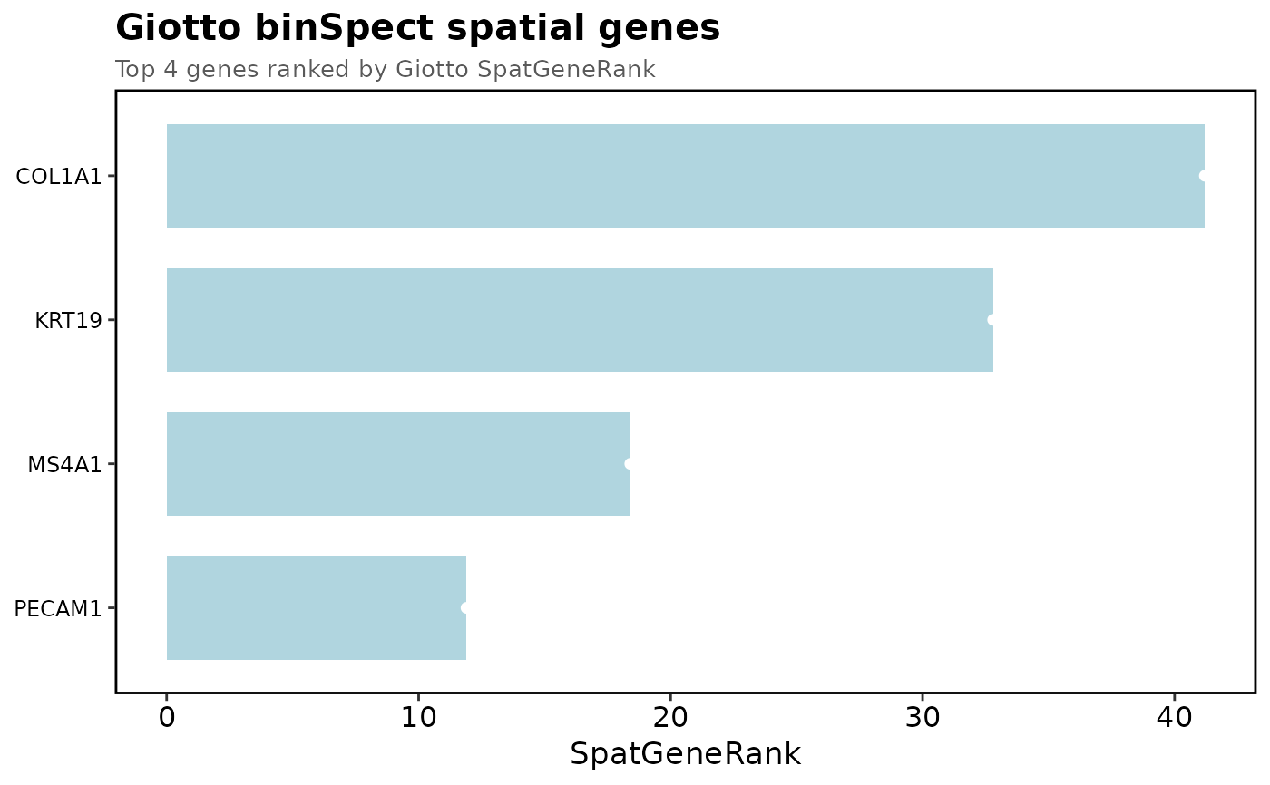
spatial_genes <- list(
  results = data.frame(
    feat_ID = c("COL1A1", "KRT19", "MS4A1", "PECAM1"),
    spatGeneRank = c(41.2, 32.8, 18.4, 11.9)
  ),
  top_features = c("COL1A1", "KRT19", "MS4A1"),
  parameters = list(assay = "Spatial", layer = "data")
)
class(spatial_genes) <- c("giotto2_spatial_genes", "giotto2_result", "list")
GiottoPlot(spatial_genes, plot_type = "ranking", top_n = 4)


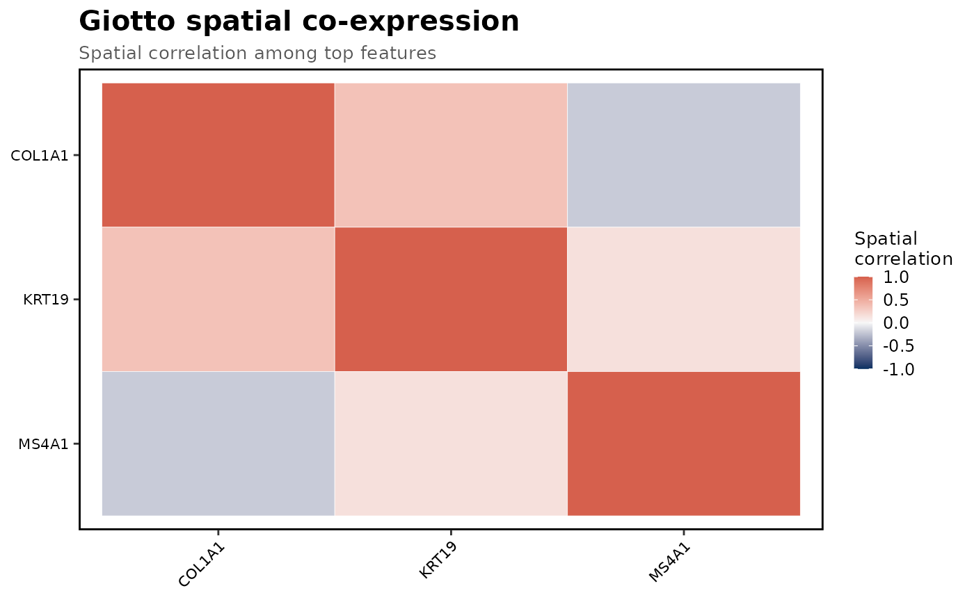
modules <- list(
  module_tables = list(
    result.cor_DT = expand.grid(
      feat_ID = c("COL1A1", "KRT19", "MS4A1"),
      variable = c("COL1A1", "KRT19", "MS4A1")
    )
  ),
  features = c("COL1A1", "KRT19", "MS4A1")
)
modules$module_tables$result.cor_DT$spat_cor <- c(
  1, 0.35, -0.20,
  0.35, 1, 0.15,
  -0.20, 0.15, 1
)
class(modules) <- c("giotto2_spatial_modules", "giotto2_result", "list")
GiottoPlot(modules, top_n = 3)