Compute Local Inverse Simpson's Index (LISI)

Compute per-cell Local Inverse Simpson's Index (LISI) scores for one or more categorical variables. This is a clean-room reimplementation of the immunogenomics/LISI.

Usage

compute_lisi(
  X,
  meta_data,
  label_colnames,
  perplexity = 30,
  tol = 1e-05,
  max_iter = 50,
  knn_algorithm = c("auto", "brute_force", "clustered"),
  n_threads = NULL,
  max_dense_bytes = Inf
)

Arguments

X

A matrix-like object with cells in rows and embedding/features in columns.

meta_data

A data frame with one row per cell.

label_colnames

Character vector of column names in meta_data to evaluate.

perplexity

Effective neighborhood size. Defaults to 30.

tol

Tolerance used in the binary search for the target perplexity. Defaults to 1e-5.

max_iter

Maximum number of binary-search iterations. Defaults to 50.

knn_algorithm

Exact nearest-neighbor search strategy. "auto" uses clustered exact search when there are at least 4096 observations and the requested neighborhood is less than one quarter of the data; otherwise it uses brute force. "brute_force" and "clustered" force either exact strategy.

n_threads

Number of C++ worker threads. NULL (the default) preserves the earlier automatic hardware-thread selection. Supply a positive integer to control CPU use explicitly.

max_dense_bytes

Maximum estimated bytes allowed for the dense input and its C++ row-major copy. The default, Inf, preserves earlier behavior; supply a finite value to enable the guard.

Value

A data frame with one row per cell and one column per label.

Details

Both nearest-neighbor strategies are exact. Sparse X is converted to a dense matrix before neighbor search; this conversion is included in the max_dense_bytes check.

References

Korsunsky I, Millard N, Fan J, et al. Fast, sensitive and accurate integration of single-cell data with Harmony. Nature Methods (2019). https://www.nature.com/articles/s41592-019-0619-0

LISI reference implementation: https://github.com/immunogenomics/LISI

Examples

set.seed(1)
X <- rbind(
  matrix(stats::rnorm(100, mean = -1), ncol = 2),
  matrix(stats::rnorm(100, mean = 1), ncol = 2)
)
meta_data <- data.frame(
  batch = rep(c("A", "B"), each = 50),
  group = sample(c("g1", "g2"), 100, replace = TRUE)
)

res <- compute_lisi(
  X, meta_data,
  c("batch", "group"),
  perplexity = 10
)
head(res)
#>      batch    group
#> 1 1.008491 1.922116
#> 2 1.001277 1.956112
#> 3 1.005979 1.747556
#> 4 1.030285 1.995189
#> 5 1.841283 1.967195
#> 6 1.484192 1.668199
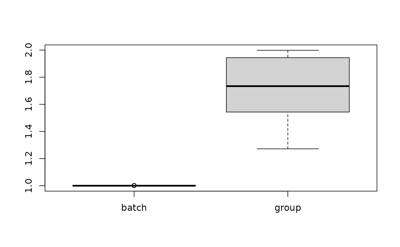
boxplot(res)